American Journal of Oper ations Research, 2011, 1, 57-64
doi:10.4236/ajor.2011.12009 Published Online June 2011 (http://www.SciRP.org/journal/ajor/)
Visualizing Investment Decision on Decision Balls
Li-Ching Ma
Department of Information Man a geme nt , N a t i onal U ni t ed Uni versi t y , Taipei
Received May 10, 2011; revised May 30, 2011; accepted June 8, 2011
Abstract
Decision makers’ choices are often influenced by visual background information. This study uses open-ended
equity funds in Taiwan to investigate three well-known optimal portfolio models, including the mean-vari-
ance, maximin, and minimization of mean absolute deviation. The optimal portfolios are then visualized on
Decision Balls to assist investors in making investment decisions. By observing the Decision Balls, investors
can see the optimal portfolios, compare the optimal weights provided by the different models, view the clus-
ter of funds, and even find substitute funds if preferred funds are not available.
Keywords: Visualization, Decision Ball, Investment decision, Portfolio
1. Introduction
Decision makers’ choices are often influenced by visual
background information [1,2]. Visual representations can
simplify complex information into meaningful patterns,
assist people in comprehending their environment, and
allow for simultaneous perceptions of parts as well as the
interrelationships between parts [3]. Visual representa-
tions are also recognized as being useful to present fi-
nancial issues. For instance, the efficient frontier [4] is a
well known visual representation used to help investors
understand relationships between risks and returns.
Several graphic methods have been developed to sup-
port the decision-making: for instance, Gower Plots to
detect any inconsistencies in a decision maker’s prefer-
ences and rank alternatives [5,6], and ELECTRE graphs
to help decision makers understand investment problems
[7]. All these methods, however, use a 2-dimensional
plane to illustrate the multidimensional data. A 2-dimen-
sional plane model cannot depict three points that do not
obey the triangular inequality (i.e. the total length of any
two edges must be larger than the length of the third edge)
neither can it display four points that are not on the same
plane [8].
The method employed here, is the Decision Ball,
which has not been used previously for visualizing port-
folio. The Decision Ball method [8,9] is based on multi-
dimensional scaling (MDS) [10,11] which has been
widely used in marketing and decision-making [12,13].
This study extends the Decision Ball method to visualize
optimal portfolios on the surface of a sphere. The dis-
tance between two securities is used to represent the cor-
relation between them: the larger the correlation, the
shorter the distance. Also, the fund with the higher return
is located closer to the North Pole. Mutual funds in Tai-
wan are taken as an example to demonstrate how to as-
sist investors visualize optimal portfolios on the Decision
Ball.
Taiwan’s mutual fund industry, which was founded in
1983, has been growing tremendously during the last
decade [14,15], with the number of mutual fund corpora-
tions increasing from 4 to 38 by 2008. In 1998, there
were only 200 funds with a total net asset value of
NT$745.97 billion. However, by January 2008, there were
523 funds with a net asset value totaling NT$2,040.91
billion. This shows that the total net asset values of funds
have almost tripled during the last decade. In Taiwan, the
mutual fund industry is dominated by individual inves-
tors who account for over 90% of the market volume. By
January 2008, over 1.84 million investors, about 8% of
Taiwan’s population, had invested in mutual funds.
This study examines 174 open-ended equity mutual
funds which were issued and invested in Taiwan’s Mar-
ket from January 2002 to December 2006. Three well-
known optimal portfolio models, including the mean- va-
riance [4], the maximin [16], and the minimization of mean
absolute deviation [17], are investigated. The optimal port-
folios are visualized on the Decision Balls. By studying the
Decision Balls, investors can then see the optimal portfo-
lios, compare the optimal weights provided by different
models, view the cluster of funds, and even find substitute
funds if the preferred funds are not available.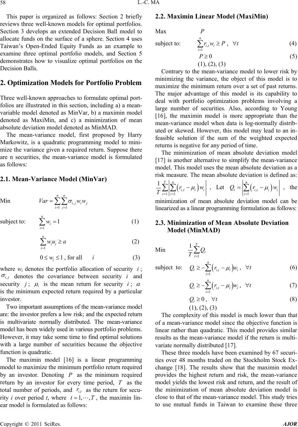

L.-C. MA 58
1
This paper is organized as follows: Section 2 briefly
reviews three well-known models for optimal portfolios.
Section 3 develops an extended Decision Ball model to
allocate funds on the surface of a sphere. Section 4 uses
Taiwan’s Open-Ended Equity Funds as an example to
examine three optimal portfolio models, and Section 5
demonstrates how to visualize optimal portfolios on the
Decision Balls.
2. Optimization Models for Portfolio Problem
Three well-known approaches to formulate optimal port-
folios are illustrated in this section, including a) a mean-
variable model denoted as MinVar, b) a maximin model
denoted as MaxiMin, and c) a minimization of mean
absolute deviation model denoted as MinMAD.
The mean-variance model, first proposed by Harry
Markowitz, is a quadratic programming model to mini-
mize the variance given a required return. Suppose there
are n securities, the mean-variance model is formulated
as follows:
2.1. Mean-Variance Model (MinVar)
Min
,
11
nn
ij ij
ij
Varw w 


subject
to: (1)
1
1
n
i
i
w



1
n
ii
i
wu a


 (2)
0
i
w, for all (3) i
where wi denotes the portfolio allocation of security ; i
,ij

denotes the covariance between security i and
security ; i j

is the mean return for security ; i

is the minimum expected return required by a particular
investor.
Two important assumptions of the mean-variance model
are: the investor prefers a low risk; and the expected return
is multivariate normally distributed. The mean-variance
model has been widely used in various portfolio problems.
However, it may take some time to find optimal solutions
with a large number of securities because the objective
function is quadratic.
The maximin model [16] is a linear programming
model to maximize the minimum portfolio return required
by an investor. Denoting as the minimum required
return by an investor for every time period, as the
total number of periods, and as the return for secu-
rity i over period t, where
PT
,it
r
1,t,
2.2. Maximin Linear Model (MaxiMin)
Max P
subject to: , (4)
,
1
n
it i
i
rw P


t
0P (5)
(1), (2), (3)
Contrary to the mean-variance model to lower risk by
minimizing the variance, the object of this model is to
maximize the minimum return over a set of past returns.
The major advantage of this model is its capability to
deal with portfolio optimization problems involving a
large number of securities. Also, according to Young
[16], the maximin model is more appropriate than the
mean-variance model when data is log-normally distrib-
uted or skewed. However, this model may lead to an in-
feasible solution if the sum of the weighted expected
returns is negative for any period of time.
The minimization of mean absolute deviation model
[17] is another alternative to simplify the mean-variance
model. This model uses the mean absolute deviation as a
risk measure. The mean absolute deviation is defined as:

,
11
1Tn
iti i
ti
r
T



 w, Let

,
1
n
titi
i
Qr 


i
w, the
minimization of mean absolute deviation model can be
linearized as a linear programming formulation as follows:
2.3. Minimization of Mean Absolute Deviation
Model (MinMAD)
Min
1
1T
t
t
Q
T

subject to: , (6)

,
1
n
titi
i
Qr 

 
i
w t
wt (7)

,
1
n
titi
i
Qr 

 
,
i
0
t
Q, t

(8)
(1), (2(3)
The complmodel is much lower than that
of
xamined by 67 securi-
tie
),
exity of this
a mean-variance model since the objective function is
linear rather than quadratic. This model provides similar
results as the mean-variance model if the return is multi-
variate normally distributed [17].
These three models have been e
s over 48 months traded on the Stockholm Stock Ex-
change [18]. The results show that the maximin model
provides the highest return and risk, the mean-variance
model yields the lowest risk and return, and the result of
the minimization of mean absolute deviation model is
close to that of the mean-variance model. This study tries
to use mutual funds in Taiwan to examine these three
T

, the maximin lin-
ear model is formulated as follows: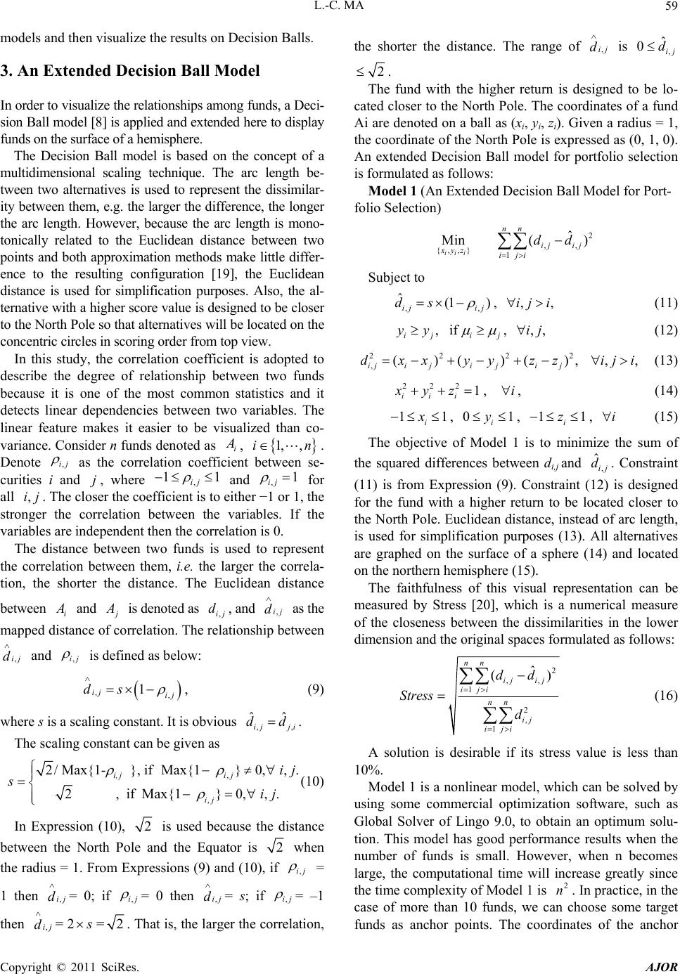

L.-C. MA59
. An Extended Decision Ball Model
order to visualize the relationships among funds, a Deci-
on the concept of a
m
opted to
de
models and then visualize the results on Decision Balls.
3
In
sion Ball model [8] is applied and extended here to display
funds on the surface of a hemisphere.
The Decision Ball model is based
ultidimensional scaling technique. The arc length be-
tween two alternatives is used to represent the dissimilar-
ity between them, e.g. the larger the difference, the longer
the arc length. However, because the arc length is mono-
tonically related to the Euclidean distance between two
points and both approximation methods make little differ-
ence to the resulting configuration [19], the Euclidean
distance is used for simplification purposes. Also, the al-
ternative with a higher score value is designed to be closer
to the North Pole so that alternatives will be located on the
concentric circles in scoring order from top view.
In this study, the correlation coefficient is ad
scribe the degree of relationship between two funds
because it is one of the most common statistics and it
detects linear dependencies between two variables. The
linear feature makes it easier to be visualized than co-
variance. Consider n funds denoted as i
A
,


1, ,in.
Denote ,ij

as the correlation coefficnt -
curities d j, where ,
11
ij
iebetween se
i an

  and ,1
ij


for
all ,ij. The closer the coefeither −, the
stror the correlation between the variables. If the
variables are
ficient is to 1 or 1
nge
sent
th
independent then the correlation is 0.
The distance between two funds is used to repre
e correlation between them, i.e. the larger the correla-
tion, the shorter the distance. The Euclidean distance
between i
A
and
j
A
is denoted as d, and ,ij d

as the
,ij
mapped dance oorrelation. The reltionshetween istf caip b
,ij
d

and ,ij

is defined as below:

,,
1
ij ij
ds

 , (9)
where s is a scaling constant. It is obvious ,,
ˆˆ
ij ji
dd.
The scaling constant can be given as
,
,
2/ Max{1- }, if Max{1 

}0, ,.
2 , if Max{1 }0, ,.
i,j ij
ij
ij
sij

 



(10)
In Expression (10), 2 is used because the distance
bee atween the North Polnd the Equator is 2 when
the radius = 1. From Expressions (9) and (10), ,ij if

=
1 then

= 0; if
,ij
d,ij

= 0 then

= s; if
,ij
d,ij

= –1
then d
s =
,ij= 22. That is, the larger the correlation,
the sh disce. The range of ,ij d

is ,
ˆ
0ij d
orter thetan
2.
fundThe with the higher return is ded
cated closer to the
Subject to
esign
2
)
to be lo-
North Pole. The coordinates of a fund
Ai are denoted on a ball as (xi, yi, zi). Given a radius = 1,
the coordinate of the North Pole is expressed as (0, 1, 0).
An extended Decision Ball model for portfolio selection
is formulated as follows:
Model 1 (An Extended Decision Ball Model for Port-
folio Selection)
,,
{,,} 1
ˆ
in (
iii ij ij
xyz iji
dd



M
nn
,
ˆij
ds ,
(1 )
ij

 , ,,ij i

 (11)
, if
ij i
yy j


, ,,ij (12)
22
,()( )( iji jiji
dxxyy z 
22
),
j
z,,ij i (13)
222
1 ,
iii
x
yz i

  , (14)
11
i
x

, 0
i
y1

, 11
i
z , i (15)
The objectivef Model ini
th
o1 is to mizthe sum of me
12)
e squared differences between di,j and ,
ˆij
d. Constraint
(11) is from Expression (9). Constraint ( is designed
for the fund with a higher return to be located closer to
the North Pole. Euclidean distance, instead of arc length,
is used for simplification purposes (13). All alternatives
are graphed on the surface of a sphere (14) and located
on the northern hemisphere (15).
The faithfulness of this visual representation can be
measured by Stress [20], which is a numerical measure
of the closeness between the dissimilarities in the lower
dimension and the original spaces formulated as follows:
2
ˆ
()
nndd
 ,,
1
2
,
1
ij ij
iji
nn
ij
iji
Stress
d




A solution is desirable if its stress value is less t
10
in
(16)
han
%.
Model 1 is a nonlinear model, which can be solved by
using some commercial optimization software, such as
Global Solver of Lingo 9.0, to obtain an optimum solu-
tion. This model has good performance results when the
number of funds is small. However, when n becomes
large, the computational time will increase greatly since
the time complexity of Model 1 is 2 n. In practice, in the
case of more than 10 funds, we can choose some target
funds as anchor points. The coordates of the anchor

L.-C. MA 60
iwan
Open-Ended Equity Funds
Th funds, which were
sued and invested in the Taiwan Market from January
1 ~ 30) and
re
30 funds. However, the MaxiMin
m
lio
points are calculated first, and then the coordinates of the
remaining funds can be obtained by calculating the cor-
relations between those funds and the anchor points.
Thus, all funds can be displayed on the Decision Ball
within a tolerable time frame.
4. Empirical Study of Ta
is study takes 174 open-ended equity
is
2002 to December 2006 for example to investigate the
three optimization models. From these 174 funds, 39
funds are excluded for the following two reasons: 1) 9
funds were not listed at the starting period 2) 30 funds
left for various reasons over the examined time period.
The monthly returns and rankings of the 135 open-ended
equity funds are listed in Table 1. Fund number 129 has
the highest monthly return of 0.0170; whereas, fund num-
ber 46 yields the lowest return, –0.0014. The average
monthly return of the 135 funds is 0.0078.
To simplify, suppose our investors are only interested
in the top 30 performance funds (i.e., rank
quest monthly returns of at least 1%, and short selling
is not allowed. The descriptive statistics for the top 30
funds are listed in Table 2. The third, fourth, fifth, and
sixth columns of Table 2 show the mean of the monthly
return, the standard deviation, and both the minimum and
maximum values of the funds. The last column describes
the ranking of funds.
The MinVar, MaxiMin, and MinMAD models are all
examined using the top
odel yields infeasible solutions. The reason is that all
top 30 funds exhibited negative monthly returns in some
months. For instance, in September 2002, affected by that
year’s stock market downturn across the United States,
Europe, and Asia, the average monthly return of the top
30 funds was –0.0892 ranging from –0.1242 to –0.0577.
The results of the MinVar and MinMAD models are
listed in Table 3. Only those funds which appear in portfo-
s at least once, i.e. the funds numbering 12, 86, 129, and
133, are shown. The weights of the funds in an optimal
portfolio for four different

are exhibited. Because

ranging from 1% to 1.3% yields the same portfolio weights,
%3.10.1 

is presentefor short. Also, since the
maximum mean of monthly returns for the top 30 funds is
, 0.01695), %7.1
d
0.0170 (exactly

is neglected be-
cause none of top 30 funds yields the mean of monthly
returns greater than or equal toe bottom two rows
of Table 3 indicate the portfolio return and variance.
As shown in Table 3, the portfolio weights in both the
MinVar and MinMAD models remain unchanged for lo
1.7%. Th
w

values ranging from 1.0% to 1.3%. In this range, the
MinVar model yields an optimal portfolio return of
132, a variance of 0.0023, and weights w86 = 0.053,
w129 = 0.243, and w133 = 0.704. Whereas, the MinMAD
model yields an optimal portfolio return of 0.0130, a
portfolio variance of 0.0023, and portfolio weights w129 =
0.219 and w133 = 0.781. As we can see, the MinVar
model provides a higher expected return than required,
and higher also than that of the MinMAD model. Given
0.0

= 1.4%, the MinVar and MinMAD models yield ex-
actly the same solutions with a portfolio return of 0.014,
riance of 0.0024, and with weights w129 = 0.413 and
w133 = 0.587. Given
a va

= 1.5% and 1.6%, an optimal
portfolio of the MinVar and MinMAD models consists
of the same funds witdifferent weights. The expected
portfolio return and variance are the same.
In this study, the outcome of the MinMAD model is
quite close to that of the MinVar model. Th
h
Balls
rep
is result is the
s
on Decision
ll model uses the distance be-
en two funds toresent the correlation between
sam
An
e
e as the conclusions of Papahristodoulou and Dot-
zauer [18], in which 67 shares traded on the Stockholm
Stock Exchange between January 1997 and December
2000 were examined. Both models provide optimal port-
folio suggestions. However, the investors cannot tell di-
rectly, the correlations among funds through table- list-
ing. The next section will demonstrate how to visualize
the optimal portfolio on Decision Balls.
5. Visualizing Optimal Portfolio
extended Decision Ba
tw
them, i.e. the larger the correlation, the shorter the dis-
tance. Also, the fund with the higher return is located
closer to the North Pole. At first, a correlation matrix of
funds is calculated. From Expression (9), ,
ˆij
d for all i, j
can be calculated. Since Max{1 }
,ij

 = 0.3064 for all
i, j, from Expression (10), the scaling constant s is given
as 4 in this example. If th funds being con-e number of
e funds numbered 12, 86,
sidered is small, then Model 1 can be applied directly to
yield the coordinates of all funds. However, when the
number of funds is large, the computational time for
Model 1 will increase greatly.
In order to increase computational efficiency, the four
funds listed in Table 3, i.e. th
129, and 133, can be chosen as the target funds. These
four funds, in which investors may be the most interested,
are suggested in an optimal portfolio for both the MinVar
and MinMAD models. The correlation matrix of the target
funds is calculated first. Applying Model 1 to these four
funds yields the coordinates of them, the so called anchor
points. The coordinates of funds numbered 12, 86, 129,
and 133 are {0.820, 0.565, 0.083}, {0.292, 0.365, 0.883},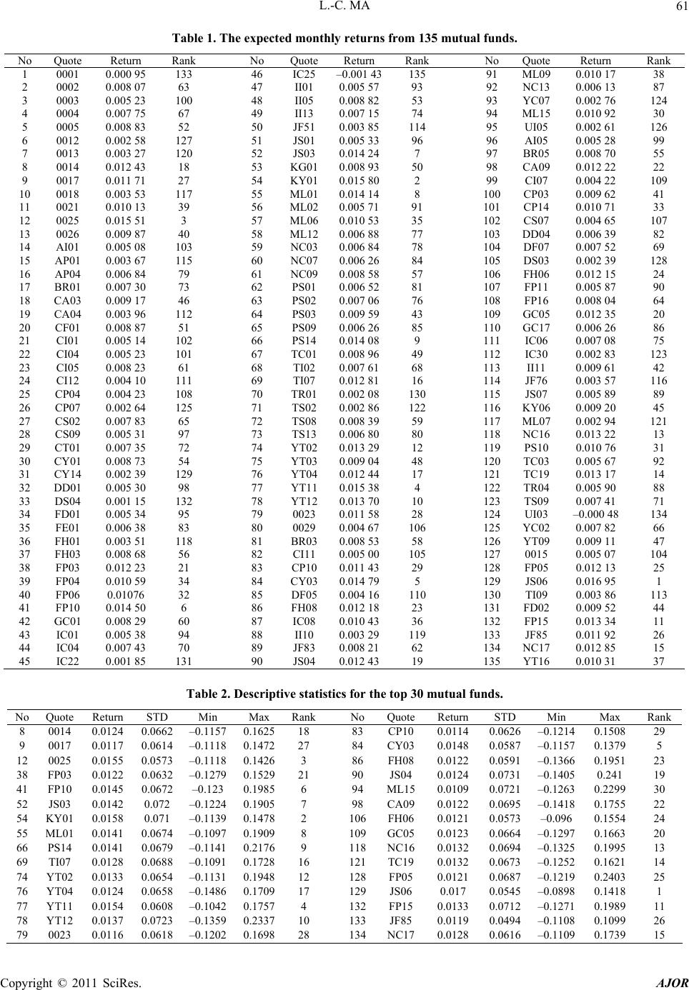

L.-C. MA61
re
No Quote Return Ran
Table 1. The expected monthlyturns from 135 mutual funds.
k
No QuoteReturnRan
k
NoQuote Return Ran
k
1 0001 0.000 95 133 46 IC25
–
0.0014313591ML09 0.010 17 38
2 0002 0.008 07 63 47 II01 0.005 57 93 92 NC13 0.006 13 87
3 0003 0.005 23 100 48 II05 0.008 82 53 93 YC07 0.002 76 124
4 0004 0.007 75 67 49 II13 0.007 15 74 94 ML15 0.010 92 30
5 0005 0.008 83 52 50 JF510.003 85 114 95 UI05 0.002 61 126
6 0012 0.002 58 127 51 JS010.005 33 96 96 AI05 0.005 28 99
7 0013 0.003 27 120 52 JS030.014 24 7 97 BR05 0.008 70 55
8 0014 0.012 43 18 53 KG010.008 93 50 98 CA09 0.012 22 22
9 0017 0.011 71 27 54 KY010.015 80 2 99 CI07 0.004 22 109
10 0018 0.003 53 117 55 ML010.014 14 8 100 CP03 0.009 62 41
11 0021 0.010 13 39 56 ML020.005 71 91 101 CP14 0.010 71 33
12 0025 0.015 51 3 57 ML060.010 53 35 102 CS07 0.004 65 107
13 0026 0.009 87 40 58 ML120.006 88 77 103 DD04 0.006 39 82
14 AI01 0.005 08 103 59 NC030.006 84 78 104 DF07 0.007 52 69
15 AP01 0.003 67 115 60 NC070.006 26 84 105 DS03 0.002 39 128
16 AP04 0.006 84 79 61 NC090.008 58 57 106 FH06 0.012 15 24
17 BR01 0.007 30 73 62 PS010.006 52 81 107 FP11 0.005 87 90
18 CA03 0.009 17 46 63 PS020.007 06 76 108 FP16 0.008 04 64
19 CA04 0.003 96 112 64 PS030.009 59 43 109 GC05 0.012 35 20
20 CF01 0.008 87 51 65 PS090.006 26 85 110 GC17 0.006 26 86
21 CI01 0.005 14 102 66 PS140.014 08 9 111 IC06 0.007 08 75
22 CI04 0.005 23 101 67 TC010.008 96 49 112 IC30 0.002 83 123
23 CI05 0.008 23 61 68 TI020.007 61 68 113 II11 0.009 61 42
24 CI12 0.004 10 111 69 TI070.012 81 16 114 JF76 0.003 57 116
25 CP04 0.004 23 108 70 TR010.002 08 130 115 JS07 0.005 89 89
26 CP07 0.002 64 125 71 TS020.002 86 122 116 KY06 0.009 20 45
27 CS02 0.007 83 65 72 TS080.008 39 59 117 ML07 0.002 94 121
28 CS09 0.005 31 97 73 TS130.006 80 80 118 NC16 0.013 22 13
29 CT01 0.007 35 72 74 YT020.013 29 12 119 PS10 0.010 76 31
30 CY01 0.008 73 54 75 YT030.009 04 48 120 TC03 0.005 67 92
31 CY14 0.002 39 129 76 YT040.012 44 17 121 TC19 0.013 17 14
32 DD01 0.005 30 98 77 YT110.015 38 4 122 TR04 0.005 90 88
33 DS04 0.001 15 132 78 YT120.013 70 10 123 TS09 0.007 41 71
34 FD01 0.005 34 95 79 00230.011 58 28 124 UI03 –0.000 48 134
35 FE01 0.006 38 83 80 00290.004 67 106 125 YC02 0.007 82 66
36 FH01 0.003 51 118 81 BR030.008 53 58 126 YT09 0.009 11 47
37 FH03 0.008 68 56 82 CI110.005 00 105 127 0015 0.005 07 104
38 FP03 0.012 23 21 83 CP100.011 43 29 128 FP05 0.012 13 25
39 FP04 0.010 59 34 84 CY030.014 79 5 129 JS06 0.016 95 1
40 FP06 0.01076 32 85 DF050.004 16 110 130 TI09 0.003 86 113
41 FP10 0.014 50 6 86 FH080.012 18 23 131 FD02 0.009 52 44
42 GC01 0.008 29 60 87 IC080.010 43 36 132 FP15 0.013 34 11
43 IC01 0.005 38 94 88 II10 0.003 29 119 133 JF85 0.011 92 26
44 IC04 0.007 43 70 89 JF830.008 21 62 134 NC17 0.012 85 15
45 IC22 0.001 85 131 90 JS040.012 43 19 135 YT16 0.010 31 37
Table 2. Descriptive statistics for the top 30 mutual funds.
No Quote Return STD Min Max RankNo QuoteReturn STD Min Max Rank
8 0014 0.0124 0.0662–0.1157 0.162518 83 CP10 0.0114 0.0626 –0.1214 0.150829
9 0017 0.0117 0.0614–0.1118 0.147227 84 CY030.0148 0.0587 –0.1157 0.13795
12 0025 0.0155 0.0573–0.1118 0.14263 86 FH08 0.0122 0.0591 –0.1366 0.195123
38 FP03 0.0122 0.0632–0.1279 0.152921 90 JS04 0.0124 0.0731 –0.1405 0.241 19
41 FP10 0.0145 0.0672–0.123 0.19856 94 ML150.0109 0.0721 –0.1263 0.229930
52 JS03 0.0142 0.072–0.1224 0.19057 98 CA090.0122 0.0695 –0.1418 0.175522
54 KY01 0.0158 0.071–0.1139 0.14782 106FH06 0.0121 0.0573 –0.096 0.155424
55 ML01 0.0141 0.0674–0.1097 0.19098 109GC050.0123 0.0664 –0.1297 0.166320
66 PS14 0.0141 0.0679–0.1141 0.21769 118NC160.0132 0.0694 –0.1325 0.199513
69 TI07 0.0128 0.0688–0.1091 0.172816 121TC19 0.0132 0.0673 –0.1252 0.162114
74 YT02 0.0133 0.0654–0.1131 0.194812 128FP05 0.0121 0.0687 –0.1219 0.240325
76 YT04 0.0124 0.0658–0.1486 0.170917 129JS06 0.017 0.0545 –0.0898 0.14181
77 YT11 0.0154 0.0608–0.1042 0.17574 132FP15 0.0133 0.0712 –0.1271 0.198911
78 YT12 0.0137 0.0723–0.1359 0.233710 133JF85 0.0119 0.0494 –0.1108 0.109926
79 0023 0.0116 0.0618–0.1202 0.169828 134NC170.0128 0.0616 –0.1109 0.173915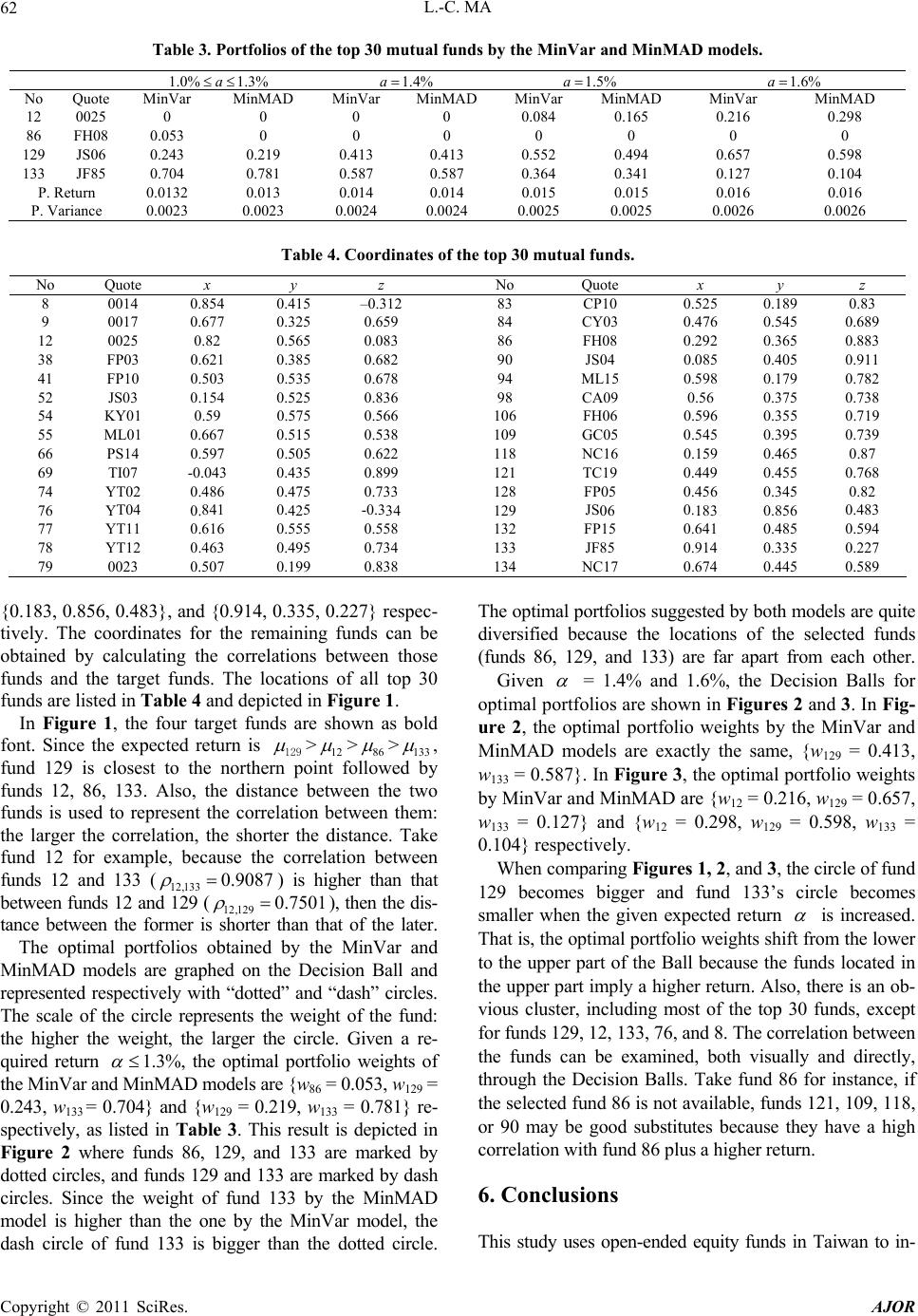

L.-C. MA 62
Table 3. P models. ortfolios of the top 30 mutual funds by the MinVar and Mi nMAD
1.0% 1.3%a 1.4%a

a1.6%a1.5%

No AD VMinnMarnMAD Quote MinVar MinMMinar inMMAD Var MiAD MinV iM
12 0025 0 0 00.084 0.165 6 0.298
00 0 0
13 0.40.552 0.494 7 0.598
87 0.50.364 0.341 27 0.104
Re0.00.00.0116 0.016
Var23 24 00.0000226 0026
0 0.21
86 FH08 0.053 0 0 0
129 JS06 0.243 0.219 0.413 0.65
133 JF85 0.704 0.781 0.587 0.1
P.turn 0.0132 0.013 0.014 14 15 5 0.0
P.iance 0.0023 0.000.000.024 25 0.5 0.000.
Table 4. Coordinates of the top 30 mutual funds.
o uotx y z Qu NQe Nootex y z
8 014854 0.5 –0. CP10 0.0.0 0.41312 83525 0.189 83
9 017677 0.5 0.6 CY03 0.0.689
025.82 0.5 0.0 FH 0.0.883
P03621 0.5 0.682 JS 0.0.911
P10503 0.5 0.678 ML 0.0.782
03154 0.5 0.8 CA09 0.0.738
Y0.59 0.5 0.566 FH 0.0.719
L0667 0.5 0.538 GC 0.0.739
S14597 0.5 0.622 NC 0.0.87
I07.043 0.5 0.8 TC 0.0.768
T02486 0.5 0.733 FP 0.0.82
T04841 0.5 -0.3 JS 0.0.483
T11616 0.5 0.558 FP 0.0.594
T12463 0.5 0.734 JF 0.0.227
023507 0.9 0.8 NC17 0.0.589
0 0.3259 84476 0.545
12 0 05683 8608292 0.365
38 F 0.38 9004085 0.405
41 F 0.53 9415598 0.179
52 JS 0.5236 9856 0.375
54 K1 057 10606596 0.355
55 M1 0.51 10905545 0.395
66 P 0.50 11816159 0.465
69 T -04399 12119449 0.455
74 Y 0.47 12805456 0.345
76 Y 0.4234 12906183 0.856
77 Y 0.55 13215641 0.485
78 Y 0.49 13385914 0.335
79 0 0.1938 134674 0.445
{0., 04 {0., 0.5, 07} -
tiv Tdr thmaingds
obtainedlcue beene
funantars. The locationsall 0
funds are listed in and ict in Fre
g thrgedsre sn d
fon inex
183.856, 0.83}, and91433.22respec
ely.he coorinates foe rein funcan be
by calating thcorrelationsetw thos
ds d the get fund of top 3
Table 4dep edigu1.
In Fiure 1,e four tat fun ahowas bol
t. Sc e thepected return is 129  >12

>86

>133

,
y
o
between
fund 129 is closest to the no
fun12133the
funds is used to represent the correlation :
the largeorthe
fund 12 xamause the c
133
rthern po
anc
rter h
7
int
betw
e
rrelation
follow
n th
between them
distance. Take
ed b
ds , 86, . Also, disteeee tw
rc the relation, sho t
for eple, beco
funds 12 and (12,133 0.908


nd 129 (12,129
) s
0.75
i hig
01
her than that
etween funds 12 ab

), then the dis-
tance between the for
th
MiAand
represented respy dotted” and “dash” circles.
Thath rtithe d:
thegh tecene-
quired return
mer is shorter than that of the later.
The optimal portfolios obtained bye MinVar and
nMD models are graphed on the Decision Bll a
ectivelwith “
e scle of e circleepresens the weght of fun
hier the weight,he larg r the cir le. Giv a r


1.3%, ptof
the ndADel863, w9 =
0.243, w.d =.781 re-
sp e listed in T. upicted in
Fie r ,arked by
dotted circles, asd bysh
cir. thnin
mo ehbynodel, the
dash circle of f3ghd le.
opti portliogey bls arite
rsifiecae oc of
s 8, nd aap
iven
the oimal portfolio weights
MiVar an MinM mods are {w = 0.0512
133 = 0704} an {w129 0.219, w133 = 0}
ectivly, asable 3This reslt is de
gur2 whee funds 86, 129 and 133 are m
nd fund 129 an 133 are marked da
clesSince he weigt of fud 133 by the MMAD
del is highr than te one the MiVar m
und 13 is biger than te dottecirc
The malfos sugsted both modee qu
diveed busthe lations the selected funds
(fund6, 129a133)re far art from each other.
G

= 4% 1the Bfor
alfoli arigu d 3. ig-
2, ttiml pliotsinVnd
Aode araca = 13,
= 0.In Fig , the optimlio w
inVnd MinM a = 129 =7,
= 07} and {, w8, 3 =
4} rctivy.
henparing F esnd rcle of fund
becomes bigger ad 133’ses
ted return
1. and.6%, Decisionalls
optim portose shown in Fres 2 anIn F
ure he opaortfo hweig by the Mar a
MinMD mlse extly the sme, {w129 0.4
w133 587}. ure 3al portfoeights
by Mar aADre {w12 0.216, w 50.6
w133 .12w12 = 0.298129 = 0.59w13
0.10espe el
W
129
comigur
n
1, 2, a
fund
3, the ci
circle becom
smaller when the given expec

is increased.
weights shift from the lower
ther thbecause the funds located in
e upar a rlse is ob-
ouerin op ds, except
r fu293d 8. The corn ben
e caxa uad dtly,
roe D a 8nsta, if
e sd f isan, 1018,
9s because they have a high
rr w 8aet
. Cus
his us-qswanin-
That is, the optimal portfolio
toe upppart of e Ball
thpper t imply highereturn. Ao, theran
vis clust, includg mostf the to30 fun
fonds 1, 12, 13, 76, anrelatioetwe
thfunds n be emined, both vislly anirec
thugh thecision Balls. Tkde fun6 for ince
thelecteund 86 not avilable, fuds 1219, 1
or0 may be good substitute
coelationith fund6 plus higher rurn.
6onclions
T studyes open ended euity fund in Tai to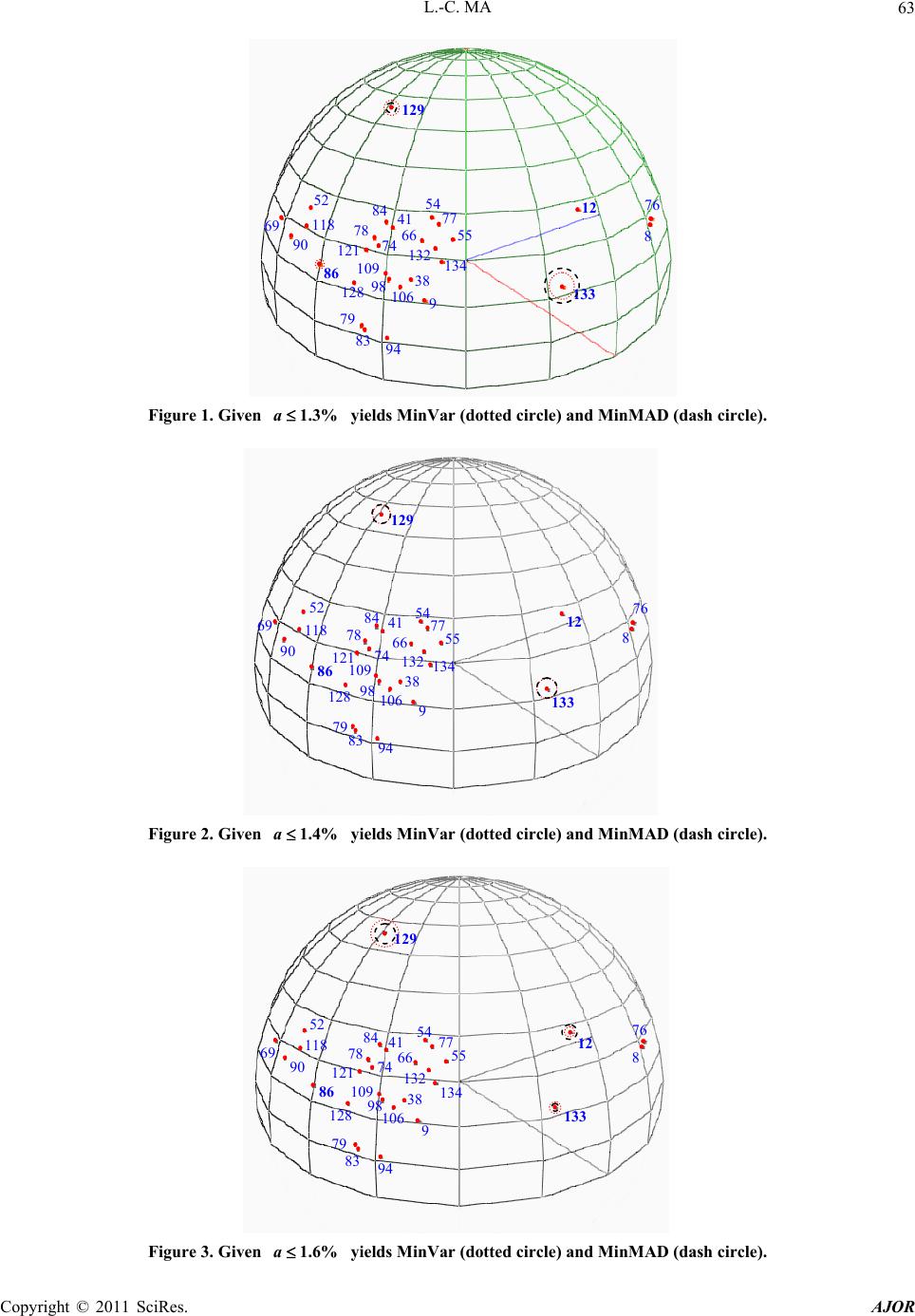

L.-C. MA63
en yields MinVar (dotircle) anAD (ircle
r (d
(d
Figure 1. Giv1.3%a ted cd MinMdash c).
otted circle) and MinM AD (dash ci rcle). Figure 2. Given 1.4%a yields MinVa
Figure 3. Given 1.6%a yields MinVarotted circle) and M i nMAD (dash circle).
94
83
79 9
134
54 77
66
132
106
38
98
109
128
121 74
78
84
129
86
52
118
90
69 41
133
12 8
76
55
94
8
79
1
12
8
9
55 66
38
12
78
129
86
52
118 41
3
33
54
77 76
134
132
109
121 74
90
84
69
106
8 98
9 4
83
79
9
55
134
54
77
66
132
106
38
98
109
128
121 74
78
84
86
52
118
90
69 41
133
129
12
8
76

L.-C. MA 64
vestigate three well-known optimal portfolio models, in-
cluding the mean-variance, maximin, and minimization of
mean absolute deviation. The maximin model yields infea-
sible solutions because all top 30 funds exhibit neg
monthly returns in some months during the examined time
period. The outcome of the minimization of mean absolute
deviation model is quite close to that of theiance
model. This result is the same as the cosion
study by Papahristodoulou and Dotzauerih-
curities traded on the Stockholm StoEx
examined. An extended Decision Ball model is proposed to
visualize optimal portfolios on the surface
where the distance between two funds indicates the corre-
lation between them, and the fund with a highn is
located closer to the North Pole. The scale of optimal port-
folio weights is represented by the size of the circle of the
selected fund. By ocision Ba
n see the optimal portfolio, compare the optimal weights
provided by the different models, view the cluster of funds,
and even find substitute funds if the preferred funds are not
available. In future studies, the question of how to linearize
this non-linear model in order to general a global oal
solution can be addressed.
7. References
[1] I. Simonson and A. Tversky, “Cot:de
off Contrast and Extremeness Aversi
Marke ting Research, Vol. 29, No. 3, 1992, pp. 281-2
doi:10.2307/3172740
ative
mean-var
nclus for the
[
ck
18], n wic
e w
h se
changere
of a sphere,
er retur
bserving the Dells, investors
ca
ptim
hoice in Cntex Tra-
on,” Journal of
95.
[2] L. M. Seiford and J. Zhu, “Context-Dependent Data En-
velopment Analysis—Measuring Attractiveness and Pro-
gress,” Omega, Vol. 31, No. 5, 2003, pp. 397-408.
doi:10.1016/S0305-0483(03)00080-X
[3] A. Meyer, “Visual Data in Organizational Research,”
Organization S
] H. Markowitz, “Portfolio Selection,” Journal of Finance,
Vol. 7, No. 1, 1952, pp. 77-91. doi:10.2307/2975974
cience, Vol. 2, No. 2, 1991, pp. 218-236.
[4
[5] C. Genest and S. S. Zhang, “A Graphical Analysis of
Ratio-Scaled Paired Comparison Data,” Management
Science, Vol. 42, No. 3, 1996, pp. 335-349.
doi:10.1287/mnsc.42.3.335
[6] L. C. Ma and H. L. Li, “Using Gower Plots and Decision
Balls to Rank Alternatives Involving Inconsistent Prefer-
ences,” Decision Support Systems, Vol. 51, N, 20
pp. 712-719. doi:10.1016/j.dss.2 .0
o. 311,
011 4.004
[7] B. P. Gladish, D. F. Jones, M. Ta
“An Interactive Three-Stage Model foFs
Portfolio Selection,” Omega, Vol. 35, No. 1, 2007, pp.
75-88. doi:10.1016/j.omega.2005.04.003
miz and A.
utua
B. Terol,
r Ml und
[8] H. L. Li and L. C. Ma, “Visualizing Decision Processes
on Spheres Based on the Even Swap Concept,” Decision
Support Systems, Vol. 45, No. 2, 2008, pp. 354-367.
[9] L. C. Ma, “Visualizing Preferences on Spheres for Group
Decisions Based on Multiplicative Preference Relations,”
European Journal of Operational Research, Vol. 203, No.
1, 2010, pp-184. doi:10.1016/j.ejor.2009.07.008. 176
[10] I. Borg and P. Groenen, “Modern Multidimensional
Scaling,” Springer, New York, 1997.
[11] T. F. Cd M. A. A. Cox, “Multidimensional Scaling
on a Sphere,” Communications on Statistics: Theory and
Methods, Vol. 20, No. 9, 1991, pp. 2943-2953.
doi:10.1080/03610929108830679
ox an
[12] W. S. Desarbo and K. Jedi, “The Spatial Representation
Marketing Sci-
doi:10.1287/mksc.14.3.326
di
Of Heterogeneous Consideration Sets,”
ence, Vol. 14, No. 3, pp. 326-342.
[13] R. L. Andrews and A. K. Manrai, “MDS Maps For Prod-
uct Attributes and Market Response: An Application to
Scanner Panel Data,” Marketing Science, Vol. 18, No. 4,
1999, pp. 584-604. doi:10.1287/mksc.18.4.584
[14] P. G. Shu, Y. H. Yeh and T. Yamada, “The Behavior of
Taiwan Mutual Fund Investors-Performance and Fund
Flows,” Pacific-Basin Finance Journal, Vol. 10, No. 5,
2002, pp. 583-60/S0927-538X(02)00070-70. doi:10.1016
[15] C. S. Hsu and“Mutual Fund Performance and
Persistence in Taiwan: A Non-Parametric Approach,”
The Service Industries Journal, Vol. 27, No. 5, 2007, pp.
509-523. doi:10.1080/02642060701411658
J. R. Lin,
[16] M. R. Young, “A Minimax-Portfolio Selection Rule with
Linear Programming Solution,” Management Science,
Vol. 44, No. 5, 1998, pp. 673-683.
doi:10.1287/mnsc.44.5.673
[17] H. Konno and H. Ya, “Mean-Absolute Deviation
Application to To-
nce, Vol. 37, No. 5,
1991, pp. 519-531. doi:10.1287/mnsc.37.5.519
mazaki
Portfolio Optimization Model and Its
kyo Stock Market,” Management Scie
[18] C. Papahristodoulou, and E. Dotzauer, “Optimal Portfo-
lios Using Linear Programming Models,” Journal of the
Operational Research Society, Vol. 55, No. 11, 2004, pp.
1169-1177.
[19] T. F. Cox and M. A. A. Cox, “Multidimensional Scal-
ing,” CRC Press, Boca Raton, 2000.
doi:10.1201/9781420036121
[20] J. B. Kruskal, “-Metric Multidimensional Scaling: A
Numericaleth” Psychometrica, Vol. 29, No. 2, 1964,
pp. 115-129. doi:10.1007/BF02289694
Non
Mod,
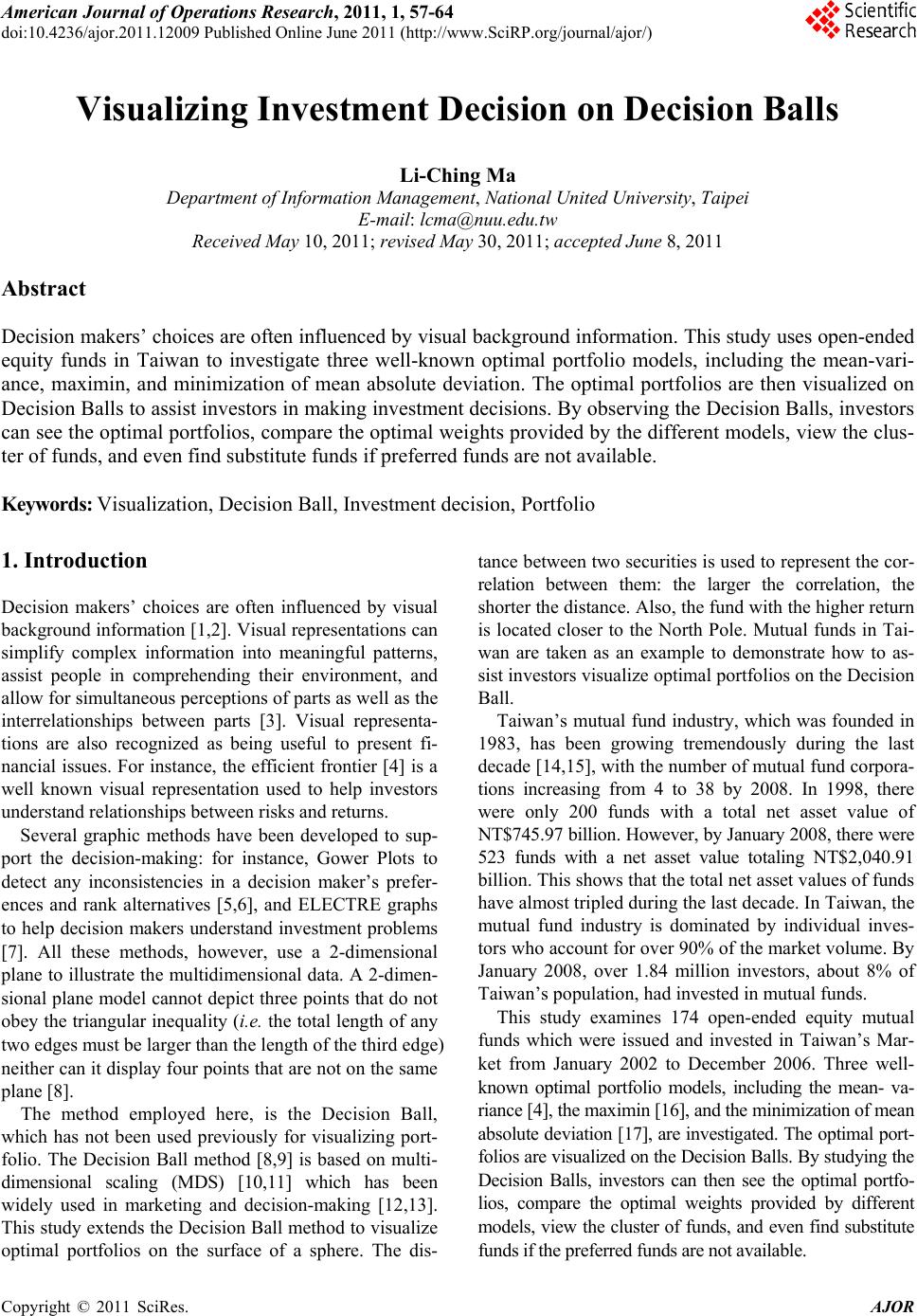