Paper Menu >>
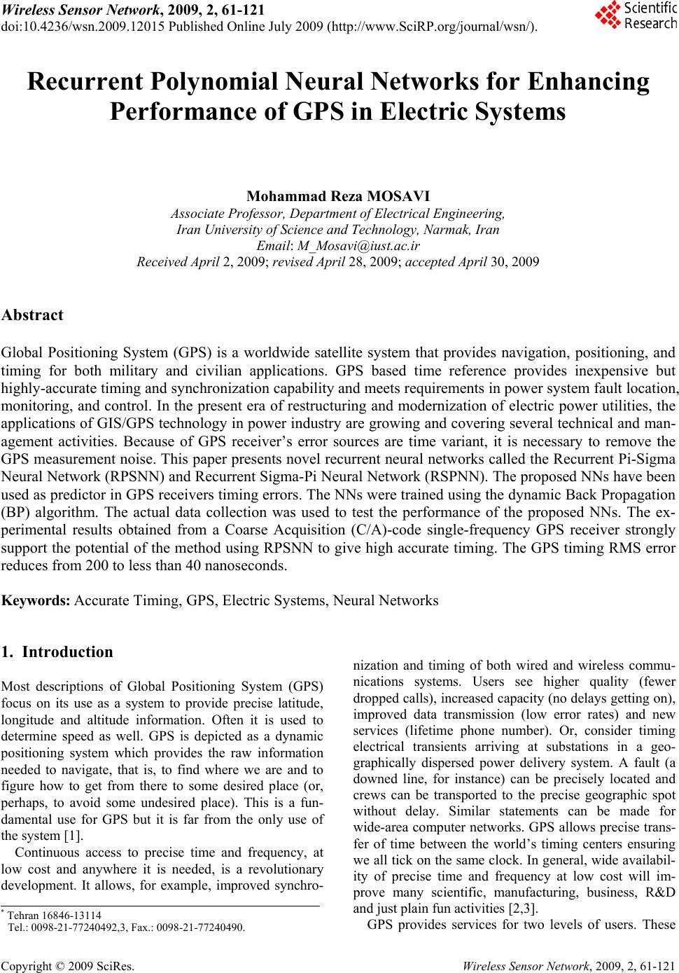
Journal Menu >>
 Wireless Sensor Network, 2009, 2, 61-121 doi:10.4236/wsn.2009.12015 Published Online July 2009 (h ttp://www.SciRP.org/journal/wsn/). Copyright © 2009 SciRes. Wireless Sensor Network, 2009, 2, 61-121 Recurrent Polynomial Neural Networks for Enhancing Performance of GPS in Electric Systems Mohammad Reza MOSAVI Associate Professor, Department of Electrical Engineering, Iran University of Science and Technology, Narmak, Iran Email: M_Mosavi@iust.ac.ir Received April 2, 2009; revised April 28, 2009; accepted April 30, 2009 Abstract Global Positioning System (GPS) is a worldwide satellite system that provides navigation, positioning, and timing for both military and civilian applications. GPS based time reference provides inexpensive but highly-accurate timing and synchronization capability and meets requirements in power system fault location, monitoring, and control. In the present era of restructuring and modernization of electric power utilities, the applications of GIS/GPS technology in power industry are growing and covering several technical and man- agement activities. Because of GPS receiver’s error sources are time variant, it is necessary to remove the GPS measurement noise. This paper presents novel recurrent neural networks called the Recurrent Pi-Sigma Neural Network (RPSNN) and Recurrent Sigma-Pi Neural Network (RSPNN). The proposed NNs have been used as predictor in GPS receivers timing errors. The NNs were trained using the dynamic Back Propagation (BP) algorithm. The actual data collection was used to test the performance of the proposed NNs. The ex- perimental results obtained from a Coarse Acquisition (C/A)-code single-frequency GPS receiver strongly support the potential of the method using RPSNN to give high accurate timing. The GPS timing RMS error reduces from 200 to less than 40 nanoseconds. Keywords: Accurate Timing, GPS, Electric Systems, Neural Networks 1. Introduction Most descriptions of Global Positioning System (GPS) focus on its use as a system to provide precise latitude, longitude and altitude information. Often it is used to determine speed as well. GPS is depicted as a dynamic positioning system which provides the raw information needed to navigate, that is, to find where we are and to figure how to get from there to some desired place (or, perhaps, to avoid some undesired place). This is a fun- damental use for GPS but it is far from the only use of the system [1]. Continuous access to precise time and frequency, at low cost and anywhere it is needed, is a revolutionary development. It allows, for example, improved synchro- nization and timing of both wired and wireless commu- nications systems. Users see higher quality (fewer dropped calls), increased capacity (no delays getting on ), improved data transmission (low error rates) and new services (lifetime phone number). Or, consider timing electrical transients arriving at substations in a geo- graphically dispersed power delivery system. A fault (a downed line, for instance) can be precisely located and crews can be transported to the precise geographic spot without delay. Similar statements can be made for wide-area computer networks. GPS allows precise trans- fer of time between the world’s timing centers ensuring we all tick on the same clock. In general, wide availabil- ity of precise time and frequency at low cost will im- prove many scientific, manufacturing, business, R&D and just plain fun activities [2,3]. * Tehran 16846-13114 Tel.: 0098-21-77240492 , 3 , Fax.: 0098-21-77240490. GPS provides services for two levels of users. These 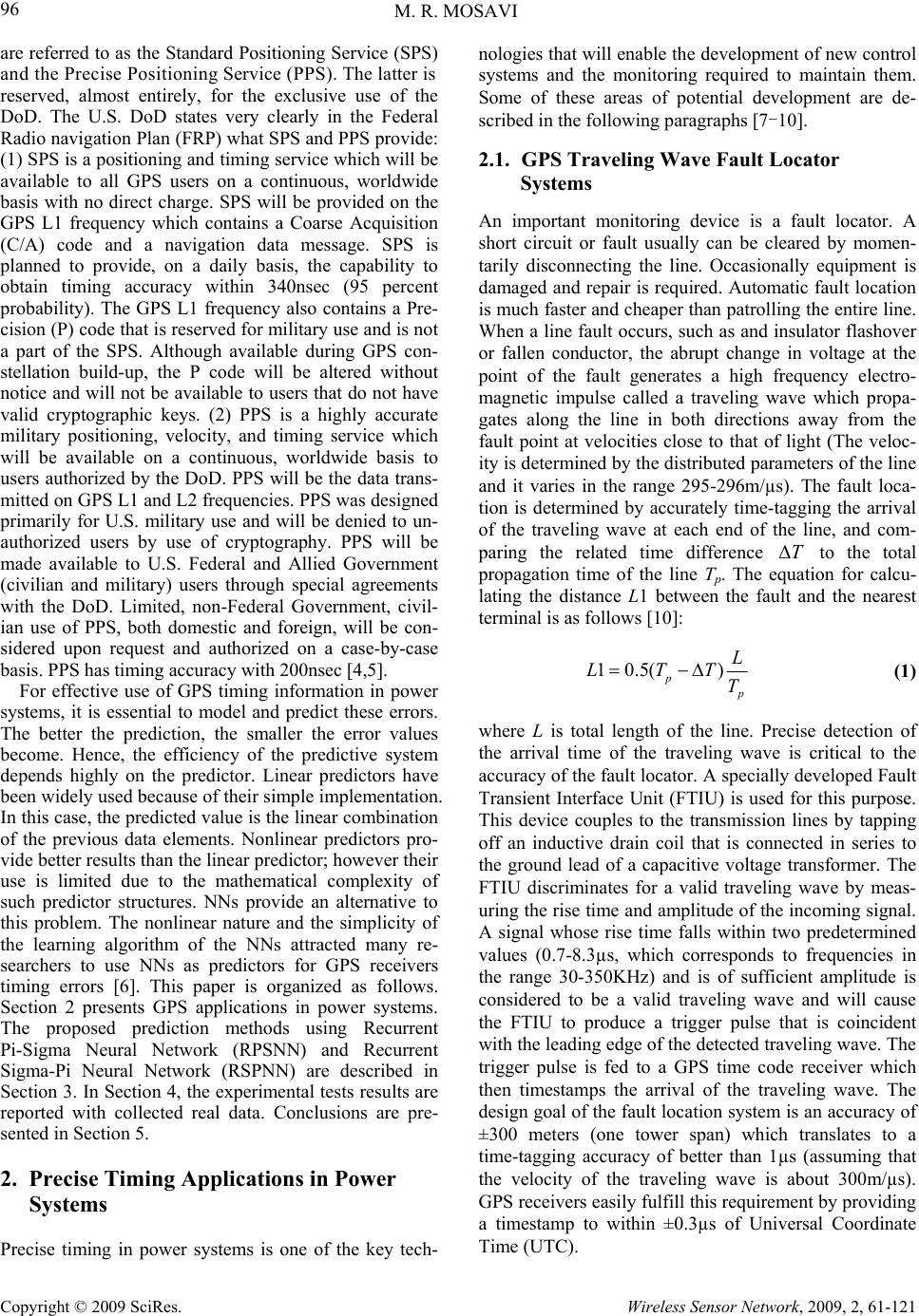 M. R. MOSAVI 96 Copyright © 2009 SciRes. Wireless Sensor Network, 2009, 2, 61-121 are referred to as the Standard Positioning Service (SPS) and th e Precise Positioning Service (PPS). The latter is reserved, almost entirely, for the exclusive use of the DoD. The U.S. DoD states very clearly in the Federal Radio navigation Plan (FRP) what SPS and PPS provide: (1) SPS is a positioning and timing serv ice which will be available to all GPS users on a continuous, worldwide basis with no direct charge. SPS will be provided on the GPS L1 frequency which contains a Coarse Acquisition (C/A) code and a navigation data message. SPS is planned to provide, on a daily basis, the capability to obtain timing accuracy within 340nsec (95 percent probability). The GPS L1 frequency also contains a Pre- cision (P) code that is reserved for military use and is not a part of the SPS. Although available during GPS con- stellation build-up, the P code will be altered without notice and will not be available to us ers that do not have valid cryptographic keys. (2) PPS is a highly accurate military positioning, velocity, and timing service which will be available on a continuous, worldwide basis to users authorized by the DoD. PPS will be the data trans- mitted on GPS L1 and L2 frequencies. PPS was designed primarily for U.S. military use and will be denied to un- authorized users by use of cryptography. PPS will be made available to U.S. Federal and Allied Government (civilian and military) users through special agreements with the DoD. Limited, non-Federal Government, civil- ian use of PPS, both domestic and foreign, will be con- sidered upon request and authorized on a case-by-case basis. PPS has timing accuracy with 200nsec [4,5]. For effective use of GPS timing information in power systems, it is essential to model and predict these errors. The better the prediction, the smaller the error values become. Hence, the efficiency of the predictive system depends highly on the predictor. Linear predictors have been widely used because of their simple implementation. In this case, the predicted value is the linear combination of the previous data elements. Nonlinear predictors pro- vide better results than the lin ear predicto r; howeve r their use is limited due to the mathematical complexity of such predictor structures. NNs provide an alternative to this problem. The nonlinear nature and the simplicity of the learning algorithm of the NNs attracted many re- searchers to use NNs as predictors for GPS receivers timing errors [6]. This paper is organized as follows. Section 2 presents GPS applications in power systems. The proposed prediction methods using Recurrent Pi-Sigma Neural Network (RPSNN) and Recurrent Sigma-Pi Neural Network (RSPNN) are described in Section 3. In Section 4, the experimental tests results are reported with collected real data. Conclusions are pre- sented in Section 5. 2. Precise Timing Applications in Power Systems Precise timing in power systems is one of the key tech- nologies that will enable the dev elopment of new control systems and the monitoring required to maintain them. Some of these areas of potential development are de- scribed in the following paragraphs [7-10]. 2.1. GPS Traveling Wave Fault Locator Systems An important monitoring device is a fault locator. A short circuit or fault usually can be cleared by momen- tarily disconnecting the line. Occasionally equipment is damaged and repair is required. Automatic fault location is much faster and cheaper than patrolling the entire lin e. When a line fault occu rs, such as and insulator flashover or fallen conductor, the abrupt change in voltage at the point of the fault generates a high frequency electro- magnetic impulse called a traveling wave which propa- gates along the line in both directions away from the fault point at velocities close to that of light (The veloc- ity is determined by th e distributed parameters of the line and it varies in the range 295-296m/µs). The fault loca- tion is determined by accurately time-tagging the arrival of the traveling wave at each end of the line, and com- paring the related time difference to the total propagation time of the line Tp. The equation for calcu- lating the distance L1 between the fault and the nearest terminal is as follows [10]: T 10.5() p p L LTT T (1) where L is total length of the line. Precise detection of the arrival time of the traveling wave is critical to the accuracy of the fault locator. A specially developed Fault Transient Interface Unit (FTIU) is used for this purpose. This device couples to the transmission lines by tapping off an inductive drain coil that is connected in series to the ground lead of a capacitive voltage transformer. The FTIU discriminates for a valid traveling wave by meas- uring the rise time and amplitude of the incoming signal. A signal whose rise time falls within two predetermined values (0.7-8.3µs, which corresponds to frequencies in the range 30-350KHz) and is of sufficient amplitude is considered to be a valid traveling wave and will cause the FTIU to produce a trigger pulse that is coincident with the leading edge of the detected trav eling wave. The trigger pulse is fed to a GPS time code receiver which then timestamps the arrival of the traveling wave. The design goal of the fault location system is an accuracy of ±300 meters (one tower span) which translates to a time-tagging accuracy of better than 1µs (assuming that the velocity of the traveling wave is about 300m/µs). GPS receivers easily fulfill this requirement by providing a timestamp to within ±0.3µs of Universal Coordinate Time (UTC).  M. R. MOSAVI 97 Copyright © 2009 SciRes. Wireless Sensor Network, 2009, 2, 61-121 The marriage of a stable atomic clock and GPS satel- lite constellation makes possible an instru ment with great accuracy and stability. It is possible to discipline a local clock with clocks of greater accuracy resident in the GPS satellite resulting in both short term and long accuracy improvements. The timing generator is a very stable and accurate instrument that has been designed to produce an accurate time standard with an absolute time accuracy of ±200nsec [11]. It has the capability of maintaining this accuracy for 24 hours after the total loss of the GPS sig- nal. Each GPS satellite contains four stable atomic clocks that are traceable to the National Institute of Standards and Technology (NIST). There are two cesium beam clocks and two rubidium clocks aboard each satellite. It is these atomic clocks which give the GPS satellite the accuracy to be used as a continual calibration source for the timing generator rubidium clock. 2.2. Sources of Synchronization Synchronization signal could be distributed over any of the traditional communication media currently in use in power systems. Most communication systems, such as leased lines, microwave, or AM radio broadcasts, place a limit on the achievable accuracy of synchronization, which is too coarse to be of practical use. Fiberoptic links, where available, could be used to provide high precision synchronization signals, if a dedicated fiber is available for this purpose. If a multiplexed fiber channel is used, synchronization errors of the order of 100 mi- croseconds are possible, and are not acceptable for power system measurements. GOES satellite systems have also been used for synchronization purposes, but their per- formance is not sufficiently accurate. The technique of choice at present is the Navstar GPS satellite transmissions. This systems is designed primar- ily for navigational purposes, but it furnishes a com- mon-access timing pulse, which is accurate to within 1 microsecond at any location on earth. The system uses transmissions from a constellation of satellites in nonsta- tionary orbits at about 10,000 miles above the earth’s surface. For accurate acquisition of the timing pulse, only one of the satellites need be visible to the antenna. The antenna is small (about the size of a water pitcher), and can be easily mounted on roof of a substation control house. The experience with the availability and depend- ability of the GPS satellite transmission has been excep- tionally good . 2.3. Phasor Measuring Units Phasor Measuring Units (PMUs) using synchronization signals from the GPS satellite system have evolved into mature tools and are now being manufactured commer- cially. The GPS receiver provides the 1 Pulse-Per-Second (PPS) signal, and a time tag, which consist of the year, day, hour, minute, and second. The time could be the local time, or the Universal Time Coordinated (UTC). The 1-PPS signal is usually divided by a phase-locked oscillator into the required number of pulses per second for sampling of the analog signals. In most systems being used at present, this is 12 times per cycle of the funda- mental frequency. The analog signals are derived from the voltage and current transformer secondaries, with appropriate anti-aliasing and su rge filtering. The microprocessor determines the positive sequence phasors according to the recursive algorithm described previously, and the timing message from the GPS, along with the sample number at the beginning of a window, is assigned to the phasor as its identifying tag. The com- puted string of phasors, one for each of the positive se- quence measurements, is assembled in a message stream to be communicated to a remote site. The messages are transmitted over a dedicated communication line through the modems. A 4800-baud communication line can sup- port the transmission of the phasor stream at the rate of about every 2-5 cycles of the fundamental frequency, depending upon th e number of p ositive sequence p hasors being transmitted. 2.4. State Estimation Modern electric utility centers use state estimators to monitor the state of the power system. The state estima- tor uses various measurements (such as complex powers and voltage and current magnitudes) received from dif- ferent substations, and, through an iterative nonlinear estimation procedure, calculates the power system state. The sate (vector) is a collection of all the positive se- quence voltage phasors of network, and, from the time the first measurement is taken to the time when the state estimate is available, several seconds or minutes may have elapsed. Because of the time skew in the data ac- quisition process, as well as the time it takes to converge to a state estimate, the available state vector is at best an averaged quasi-steady-state description of the power system. Consequently, the state estimators available in present-day control centers are restricted to steady-state applications only. Now, consider the positive sequence voltages meas- ured by the synchronized phasor measurement units. If voltages at all system substations are measured, one would have a true simultaneous measurement of the power system state. No estimation of the state vector is necessary. From a practical point of view, it is sensible to use the positive sequence currents also, which provide data redundancy. This leads to a linear estimator of the power system state, which uses both current and voltage measurements. The estimate results from the multiplica- tion, of a constant matrix by the measurement vector, and is extremely fast. In addition to a much simplified static state estimator, synchronized phasor measurements also provide the first  M. R. MOSAVI 98 Copyright © 2009 SciRes. Wireless Sensor Network, 2009, 2, 61-121 real possibility of providing a dynamic state estimator. By maintaining a continuous stream of phasor data from the substations to the control center, a state vector that can follow the system dynamics can be constructed. With normal dedicated communication circuits operating at 4800 or 9600 baud, a continuous data stream of one phasor measurement every 2-5 cycles (33.3-83.33msec) can be sustained. Considering that the usual power sys- tem dynamic phenomena fall in the range of 0-2Hz, it is possible to observe in real-time the power system dy- namic phenomena with high fidelity at the center. Another application of directly measured dynamic phenomena is to validate power system models used in transient stability studies. For the first time in history, synchronized phasor measurements have made possible the direct observation of system oscillations following system disturbances. By trying to simulate these events, one can learn a great deal about the models of major system components, and correct them as needed until the simulations and observed phenomena match well. 2.5. Improved Control Power system control elements, such as generation exci- tation systems, HVDC terminals, variable series capaci- tors, SVCs, etc., use local feedback to achieve the control objective. However, often the control objective may be defined in terms of a remote occurrence. As an example, consider the task of damping power swings between two areas by controlling (modulating) the flow on a dc line. Such a controller must have a built-in mathematical de- scription (model), which must relate the dc power to the angle between the two regions. To the extent that the assumed model is not valid under the prevailing system conditions, the controller do es not do the job for which it was intended. With synchronized phasor measurements being brought to the controller location, it becomes possible to provide direct feed-back from the angular difference between the two systems. Studies of this nature have shown that improved control performance is achieved when a model-based controller is replaced by one based upon feedba ck provided b y the phasor measurement sys- tem. 2.6. Quasi-Traveling Wave Schemes Quasi-traveling wave schemes compare only the relative phase of the charge in impedance at the inception of fault at the local end with a signal representing the relative change at the remote end. When a fault occurs, the in- stantaneous voltage will usually fall and the instantane- ous current will rise; either quantity may be positive or negative at that time. The relative change between the two represents the ch ange in impedance and the direction of the fault. The relay is triggered by a rate of change in the voltage and current and sends a directional signal. Trip decision times are short but must allow for trans- mission time of the carrier system, relative end-to-end phasing of the voltage/current is not normally critical. 3. GPS Receivers Timing Errors Modeling Using Neural Network The NN concept is used in forecasting, by considering historical data to be the input to a black box, which con- tains hidden layers of neurons. These neurons compare and structure the inputs and known outputs by nonlinear weightings, which are determin ed by a continuous learn- ing process (Back-Propagation (BP)). The learning proc- ess continues until forecast outputs are reasonably close to known actual outputs. The structure of the black box is then used for forecasting actual future outputs. For time series forecasting the inputs are the past observations of the data series and the output is the future value. The GPS receiver’s time errors () x t t is difference between the two sequence time at time , i.e., () () x tUTODt -(1)UTOD t [12]. The NNs estimate () x t at future time 1t . 3.1. Modeling Using Recurrent Pi-Sigma Neural Network Similarly to feed-forward PSNN, the RPSNN consists of three layers, the input layer, the summing units layer and the output layer. In the output layer, the NN calculates the product of the we ighted sum of the inputs and passes the result to a nonlinear transfer function. Then the out- put of the network is fed back to the inputs. Th e NN has a regular structure and requires a smaller number of weights than conventional single-layers, High-Order Neural Networks (HONNs). The weights from the sum- ming units to the product unit are fixed at unity, which implies that the summing units layer is not hidden. The adoption of the smaller number of weights results in faster training. The order of the NN corresponds to the number of units connected to the unit. Figure 1 shows the architecture of the proposed RPSNN. Let the number of external inputs to the NN to be 2 M and the number of outputs to be 1. Let (1)yn be the output of the network at time and 1n() j x n be the jth input to the NN at time n. The overall inputs to the NN are the concatenation of () x n and and is referred to as : ()yn ()zn ();1 () 1;1 () ;2 j j x nj znj M ynjM M (2) 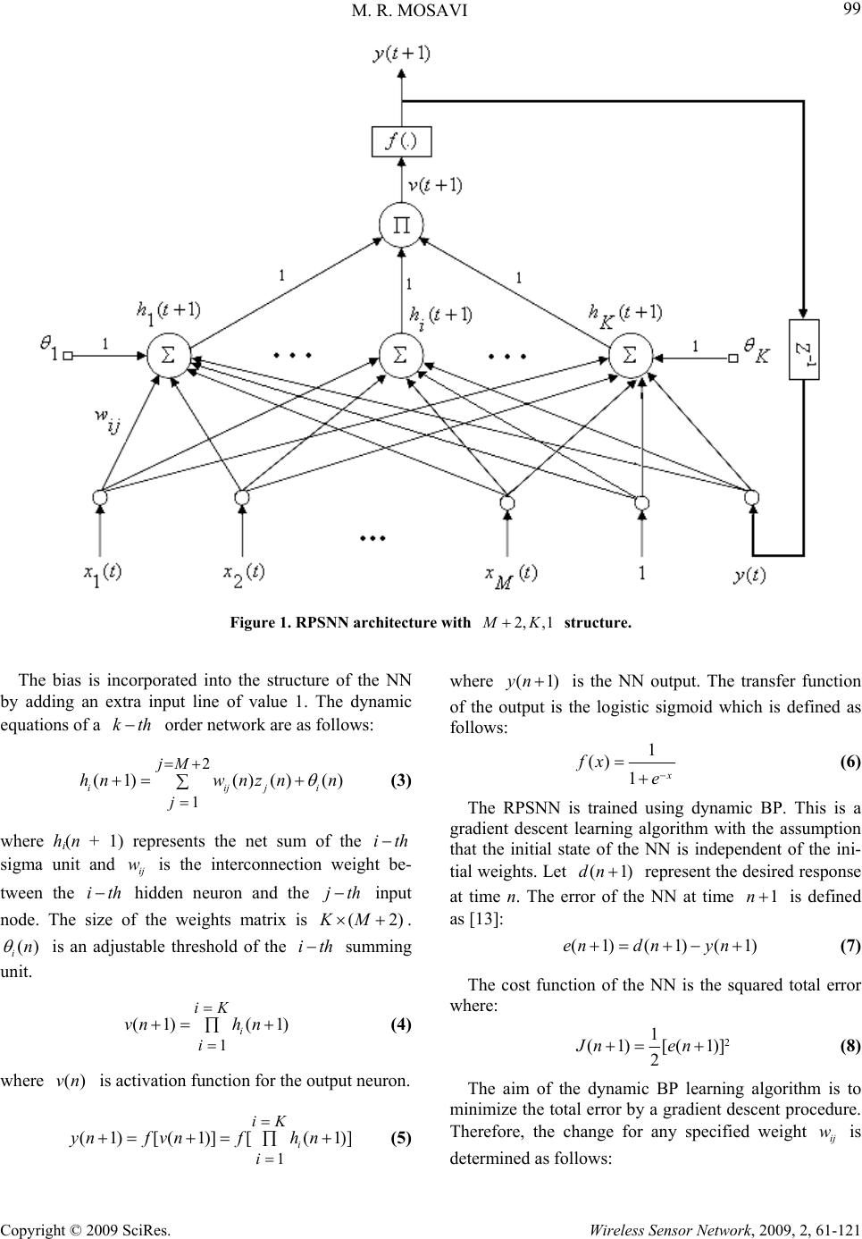 M. R. MOSAVI 99 Copyright © 2009 SciRes. Wireless Sensor Network, 2009, 2, 61-121 Figure 1. RPSNN architecture with 2, ,1 M K structure. The bias is incorporated into the structure of the NN by adding an extra input line of value 1. The dynamic equations of a order network are as follows: kth where (1)yn is the NN output. The transfer function of the output is the logistic sigmoid which is defined as follows: 1 () 1 x fx e (6) 2 1 (1)()() ( iijj jM j hnw nznn ) i (3) The RPSNN is trained using dynamic BP. This is a gradient descent learning algorithm with the assumption that the initial state of the NN is independent of the ini- tial weights. Let (1)dn represent the desired response at time n. The error of the NN at time is defined as [13]: 1n where hi(n + 1) represents the net sum of the ith sigma unit and is the interconnection weight be- tween the hidden neuron and the input node. The size of the weights matrix is . ij w hitjth KM (2) () in is an adjustable threshold of the summing unit. ith(1) (1)(1endnyn ) (7) The cost function of the NN is the squared total error where: 1 (1) (1 i iK i vnh n ) ] (4) 2 1 (1) [(1)] 2 Jn en (8) where is activation function for the output neuron. ()vn The aim of the dynamic BP learning algorithm is to minimize the total error by a gradient descent procedure. Therefore, the change for any specified weight is determined as follows: ij w 1 (1)[(1)] [(1) i iK i ynfvnfhn (5)  M. R. MOSAVI 100 Copyright © 2009 SciRes. Wireless Sensor Network, 2009, 2, 61-121 (1) (1) ( ij ij ij Jn wn wn w ) (9) where is a positive real number representing the learning rate and is the momentum term. (1) (1)(1) (1) (1) ij ijij Jn enyn en en ww w (10) In this case, (1) ij yn w is found by usin g the chain rule: (1) (1) (1) . (1)i ij iij hn yn yn whnw (11) By differentiating the dynamic equations of the NN, (1) (1) i yn hn can be obtained as follows: 11;# (1) '[(1)].[( (1) ll i lK lK llli yn fhn hn hn 1)] (12) and the value (1) i ij hn w is calculated as follows: () 2 (1) () ijij ij yn iM w hn zn w w (13) Let (1) (1) ij ij yn Pn w , then weights updating rule is: (1) (1)(1)( ijij ij wnen Pnwn) (14) With: () 2 11;# ' (1) [(1)].[(1)].[() ijll j lK lKPn iM ij llli Pnfhnhnznw ] (15) where '(.) f is the derivative of the nonlinear transfer function and is determined as follows: '()()[1 ()] f xfx fx (16) The change for any specified weight i is determined using BP learning algorithm as follows: (1) (1) ( ii i Jn nn ) (17) where (1) i Jn is obtained as: (1) (1) (1) (1) (1) i i Jn en en yn en (1) i yn is found by using the chain rule: (1) (1) (1) . (1)i ii i hn yn yn hn (19) The value (1) i i hn is calculated as follows: () 2 (1) 1 i i yn iM i hn w (20) Let (1) (1) i i yn Qn , then weights updating rule is: (1) (1)(1)() ii nenQn i n (21) i (18) With: () 2 ' (1) [(1)].[(1)].[1 11;# illQn i iM lK lK Qn fhnhnw llli ] (22) 3.2. Modeling Using Recurrent Sigma-Pi Neural Network The architecture of a RSPNN with 2 M inputs and one output is shown in Figure 2. In this network, hidden layer neurons output is the product of the input terms and the network output is the sum of these products. It also has a single layer of adaptive weights in the second layer. The RSPNN learning procedure using the BP method can be summarized as follows:  M. R. MOSAVI 101 Copyright © 2009 SciRes. Wireless Sensor Network, 2009, 2, 61-121 Figure 2. RSPNN architecture with 2, ,1 M K structure. Step1: Weight Vector Initialization Set all of the weights and thresholds of the network to small random numbers that are uniformly distributed. Step2: Forward Calculations ();1 () 1;1 () ;2 j j x nj znj M ynjM M (23) 2 1 (1)() ( ij jM j hnznn ) i ] ; i (24) 1 (1) (1) ii iK i vnwh n (25) (1) [(1)yn fvn (26) Step3: Learning Process (1) (1)(1)() ii wnen Pnwn 1 11 ' (1) [(1)]..[()].() iiiij jM iK ij PnfwhnwznPn i i (27) 1 11 (1)(1)(1)(); ' (1)[(1)]..[1(()).()] iii iiiij jM iK ij nenQnn Qnfwhnwz nQn (28) Step4: Iteration Increment time n by one unit and go back to Step2. 4. Experimental Results To test the proposed NNs for G PS r e c e iv ers timing erro rs prediction a system was built. The test setup was imple- mented and installed on the building of Computer Con- trol and Fuzzy Logic Research Lab in the Iran University of and Technology. The observation data received by a low cost and single frequency GPS receiver manufac- tured by Rockwell Company. The collected data were processed with developed programs by the paper author. Figure 3 shows the data collection system adopted in th is research. In preparing the training data, all input and output variables are normalized in the range [0,1] to reduce the training time [14]. Observation at time t is applied to NNs inputs and the networks must predict the value of instant 1t . The choice of the order for the NNs is very important in on-line prediction. It is more difficult to  M. R. MOSAVI 102 Copyright © 2009 SciRes. Wireless Sensor Network, 2009, 2, 61-121 formulate the order of a nonlinear model. In this paper, the order selection is based on the experimental results. For optimizing NNs structure, various combinations of input variables were tried. The proposed methods were implemented and developed by author of this paper using Microsoft Visual Basic6. These models were validated using a set of data points. The RPSNN and RSPNN benefit from both the ad- vantages of feed-forward HONNs and RNNs. The in- corporation of higher order terms allows the networks to make use of nonlinear interactions between the inputs, thus functionally expanding the input space into a higher-dimensional space, where linear separability, or reduction in the dimension of the nonlinearity is possible. Furthermore, the adaptation of the small number of weights allows the NNs to be trained faster than HONNs which suffer from the combinational explosion of the high-order terms and demonstrate slow learning, when the order of the NNs becomes excessively high. In con- trast to fully RNNs that are trained using the RTRL algo- rithm, the small structure of the RPSNN and RSPNN accelerates the learning of the NNs using the dynamic BP. To evaluate the performance of the presented training algorithms, they were tested by collected data sets. Six statistical measures (maximum, minimum, RMS, average, variance, standard deviation), are used to evaluate pre- diction results. Table 1 presents statistical measures on 500 test data by using the proposed NNs. In order to evaluate the prediction accuracy, we used RMS as a measure of closeness between predicted and observed values [15]. From Table 1 can be seen that time accuracy has improved by factor of about 5. Table 2 shows the comparison of test results of differ- ent models for GPS timing errors pr ediction. The simula- tion results demonstrated that RPSNN and RSPNN are efficient than PSNN,RNN and SPNN,RNN, respectively. 5. Conclusions Accurate timing using GPS can revolutionize the field of monitoring, protection, and control of power systems. It is with great excitement that we look for other applica- tions, not yet thought of, that can advance the state of the art in electric power engineering. The past few years have witnessed increasing interest in synchronized accu- rate timing and how they may be used for various power system applications. The development of new types of computer-based hardware and the completion of the GPS of satellites provide the components needed for true synchronized monitoring systems. GPS time synchroni- zation enables the accurate time tag of each recorded data sample to better than 1 microsecond accuracy. In this paper, a RPSNN and RSPNN were implemented and used as predictor in GPS system. The proposed NNs were trained using the dynamic BP, which is a gradient descent learning algorithm. The actual data collection was used to train the networks. The trained weights of the NNs were fixed and used to predict GPS receivers timing errors. Extensive tests have shown that third order NNs provide the most promising results. The tests results using the RPSNN predictor have shown an improvement in the GPS timing accuracy over the linear predictor, multilayer perceptorns, HONN s, RNNs. The GPS timing RMS error reduced from 200 to less than 40 nanosec- onds. Figure 3. Data collection and processing system. 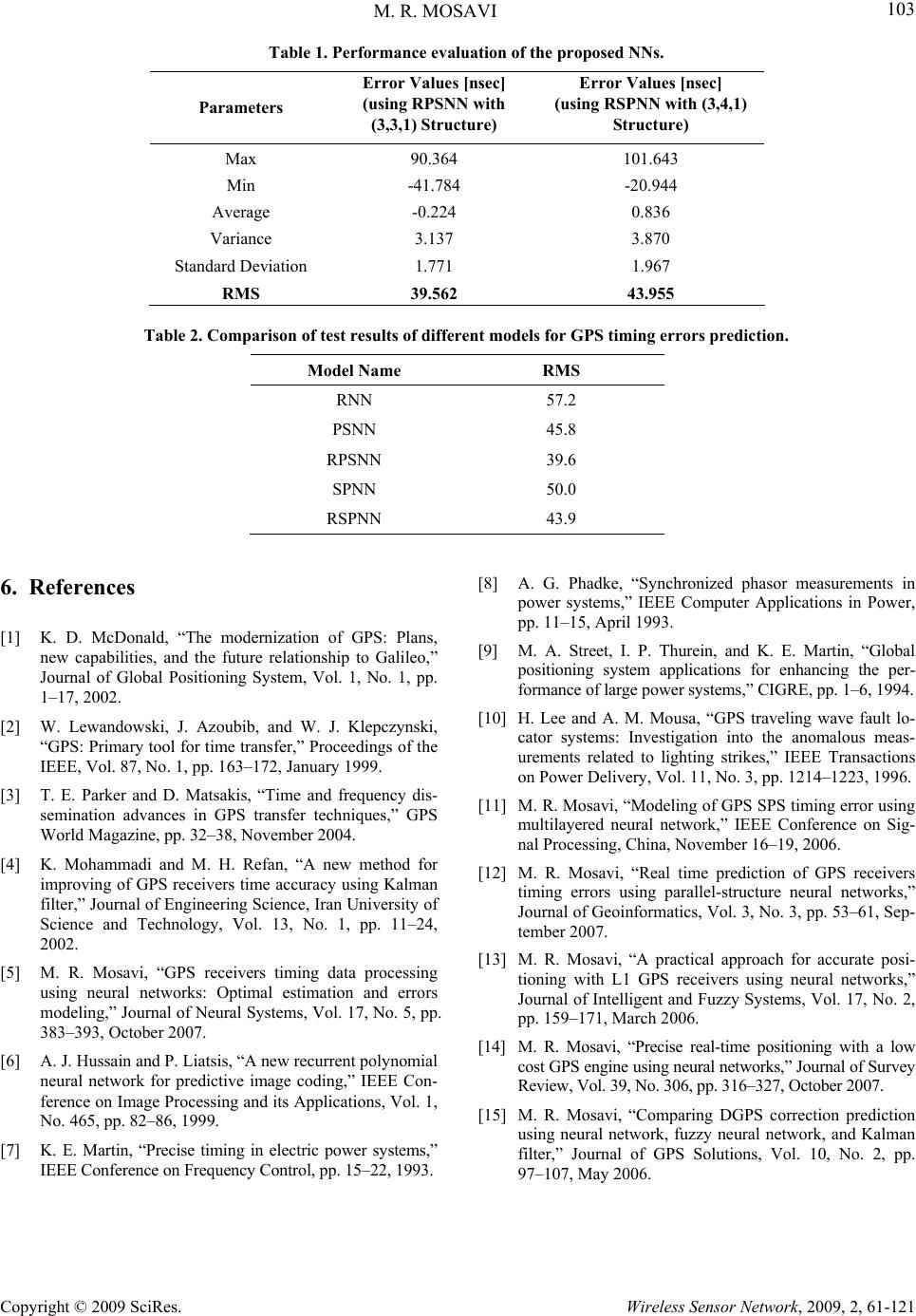 M. R. MOSAVI 103 Copyright © 2009 SciRes. Wireless Sensor Network, 2009, 2, 61-121 Table 1. Performance evaluation of the proposed NNs. Parameters Error Values [nsec] (using RPSNN with (3,3,1) Structure) Error Values [nsec] (using RSPNN with (3,4,1) Structure) Max 90.364 101.643 Min -41.784 -20.944 Average -0.224 0.836 Variance 3.137 3.870 Standard Deviation 1.771 1.967 RMS 39.562 43.955 Table 2. Comparison of test results of different models for GPS timing errors prediction. Model Name RMS RNN 57.2 PSNN 45.8 RPSNN 39.6 SPNN 50.0 RSPNN 43.9 6. References [1] K. D. McDonald, “The modernization of GPS: Plans, new capabilities, and the future relationship to Galileo,” Journal of Global Positioning System, Vol. 1, No. 1, pp. 1–17, 2002. [2] W. Lewandowski, J. Azoubib, and W. J. Klepczynski, “GPS: Primary tool for time transfer,” Proceedings of the IEEE, Vol. 87, No. 1, pp. 163–172, January 1999. [3] T. E. Parker and D. Matsakis, “Time and frequency dis- semination advances in GPS transfer techniques,” GPS World Magazine, pp. 32–38, November 2004. [4] K. Mohammadi and M. H. Refan, “A new method for improving of GPS receivers time accuracy using Kalman filter,” Journal of Engineering Science, Iran University of Science and Technology, Vol. 13, No. 1, pp. 11–24, 2002. [5] M. R. Mosavi, “GPS receivers timing data processing using neural networks: Optimal estimation and errors modeling,” Journal of Neural Systems, Vol. 17, No. 5, pp. 383–393, October 2007. [6] A. J. Hussain and P. Liatsis, “A new recurrent polynomial neural network for predictive image coding,” IEEE Con- ference on Image Processing and its Applications, Vol. 1, No. 465, pp. 82–86, 1999. [7] K. E. Martin, “Precise timing in electric power systems,” IEEE Conference on Frequency Control, pp. 15–22, 1993. [8] A. G. Phadke, “Synchronized phasor measurements in power systems,” IEEE Computer Applications in Power, pp. 11–15, April 1993. [9] M. A. Street, I. P. Thurein, and K. E. Martin, “Global positioning system applications for enhancing the per- formance of large power systems,” CIGRE, pp. 1–6, 1994. [10] H. Lee and A. M. Mousa, “GPS traveling wave fault lo- cator systems: Investigation into the anomalous meas- urements related to lighting strikes,” IEEE Transactions on Power Delivery, Vol. 11, No. 3, pp. 1214–1223, 1996. [11] M. R. Mosavi, “Modeling of GPS SPS timing error using multilayered neural network,” IEEE Conference on Sig- nal Processing, China, November 16–19, 2006. [12] M. R. Mosavi, “Real time prediction of GPS receivers timing errors using parallel-structure neural networks,” Journal of Geoinformatics, Vol. 3, No. 3, pp. 53–61, Sep- tember 2007. [13] M. R. Mosavi, “A practical approach for accurate posi- tioning with L1 GPS receivers using neural networks,” Journal of Intelligent and Fuzzy Systems, Vol. 17, No. 2, pp. 159–171, March 2006. [14] M. R. Mosavi, “Precise real-time positioning with a low cost GPS engine using neural networks,” Jour nal of Su rvey Review, Vol. 39, No. 306, pp. 316–327, October 2007. [15] M. R. Mosavi, “Comparing DGPS correction prediction using neural network, fuzzy neural network, and Kalman filter,” Journal of GPS Solutions, Vol. 10, No. 2, pp. 97–107, May 2006. |