Journal of Service Science and Management, 2011, 4, 222-226
doi:10.4236/jssm.2011.42026 Published Online June 2011 (http://www.SciRP.org/journal/jssm)
Risk Migration in Supply Chain Inventory
Financing Service
Zheng Qi n1, Xiaochao Ding2
1School of Information Management and Engineering, Shanghai University of Finance and Economics, Shanghai, China; 2Informa-
tion Engineering College of Yangzhou University, Yangzhou, China.
Received January 17th, 2010; revised March 17th, 2011; accepted April 7th, 2011.
ABSTRACT
Inventory financing affects the risks o f both for banks and supply cha in co mpa nies. Trad itio nally, su pp ly chain research
focus more on material flow than financial. We construct a supply chain financing risk-information migration model
(RMM). In this mod el , we discussed the preconditions to adopt inventory financing when the enterprises are facing cash
constraints. And we simulated th e whole operate of supply chain and bank beha vior with Matlab. The simulatio n result
shows if loan conditions are satisfied, the total risk value is reduced. Risk migration happens in the financing process.
In this process, information-risk proportions are more reasonable.
Keywords: Supply Chain, Inventory Financing, Value of Risk
1. Introduction
Modern corporate finance theory is founded on the
proposition that financial capital is supplied to firms by
investors who have an “expectation of return”, and that,
Cavinato (1991) research show supply chain can reduce
cost, improve quality and make lead time shorter [1],
thus it can improve competence of the whole supply
chain. In traditional supply chain, researchers focus more
on material flow than cash flow. It is essential to corpo-
rate supply chain research with finance theory. Recipro-
cally, such expectation represents the firm’s “cost of fi-
nancial capital” optimization along with materials in
supply chain operation. We observe that supply chain
theory begins with “irrelevancy” pronouncements about
a firm’s value being independent of its supply chain op-
timization. Risk sharing in supply chain financing, which
are ignored in most supply chain optimization, in re-
sponse to these unrealistic assumption, theoretical de-
velopment has subsequently come to be directed at pro-
viding models that are descriptive of the way corporate
financial with supply chain [2]. To this end, supply ch ain
financial has increasingly been recognized as first order.
Supply chain structure is defined as the associations
among supply chain members [3]; this structure can
benefit both vertical and horizontal connected companies
[4]. Aberdeen Group defines Supply Chain Finance (SCF)
as “a combination of Trade Financing provided by a fi-
nancial institution, a third-party vendor, or a corporation
itself, and a technology platform that unites trading part-
ners and financial institutions electron ically and provides
the financing triggers based on the occurrence of one or
several supply chain events.” Banks can offer SCF solu-
tions that enable their customers to lower costs and create
financial stability in their end-to-end supply chain-and
create deeper and broader customer relationships in the
process.
Inventory financing is a kind of supply chain finance,
which is banking line of credit secured by the company’s
inventory. Companies with tangible inventory and a
proven sales history and good credit since lenders aren't
really interested in taking possession of your inventor y if
you can't make your loan payments. John A. Buzacott &
Rachel Q. Zhang (2004) researched on the deposit and
loan decision process of supply chain companies and
banks [2]. N. R. Srinivasa Raghavan and Vinit Kumar
Mishra (2009) consider a two-level supply chain with a
single retailer and a manufacturer, where both the firms
are facing financial constraints and cannot produce/order
their optimal quantity [5].
A commonly held opinion is that the low level of
long-term profit rates could be largely explained by a
decline in the compensation for risk. This opinion is
The work is supported by China National Nature Science Foundation
under Grant 70971083.

Risk Migration in Supply Chain Inventory Financing Service 223
supported by a great deal of empirical work devoted to
the measurement of bond risk premium and the analysis
of their dynamics [6]. While financing a firm, although a
lender tries to perceive its exposure to default risk by
looking into borrower’s accounts, due to lack of proper
information, the buying or selling cap acities of preceding
or following stakeholders, as in manufacturer and its re-
tailer of supply chain remain unkn own. Lend er’s analysis
is then based on certain assumptions. This lack of infor-
mation is a reality, especially fo r small firms that are not
publicly listed.
The paper is organized as follows. In Section 2 we in-
troduce basic notation, terminology and assumptions.
The risk information migration model RMM model and
solutions is presented in Section 3. We discuss inference
and parameter estimation for RMM and presented ex-
periment results in Section 4. Finally, Section 5 presents
our conclusions.
2. Assumptions, Notations
For simplicity we assume that both the firms have no
other assets but the cash available with them before they
commence their respective activities. Both manufacture
and retailer have no fix asset such as land, buildings,
machines etc. Account payable, account receivable, cash,
inventory and short term borrowing are considered in the
model. r
q are predicted based on constant elasticity
form. The expected quantity of production is equal with
mathematical expectation of r
q (

mr
qEq
). Because
of cash constrain ts and ability to get loan from bank, real
quantity is less than expected quantity. Manufacture
firstly predicts the retailer’s purchasing before producing,
and decides a price m
p of finished product. Based on
the cash constraints of manufacture, im
L will be decided.
Bank will evaluate the risk and give a max loan available
for bank. Retailer predicts a market demand and purchase
from manufacture. At any time, cash owned by manu-
facture and retailer greater than zero, or they will bank-
rupt.
VaR is adopted to calculate risk value of manufacture
and bank loan. It is equal the maximum loss from the
specific confidence level. Based on Jorion, 1997, we can
calculate VaR with Equations (1) and (2) [7].

*
L
LL
VaR E   (1)

*
M
MM
VaR E   (2)
A simple two-stage supply chain is considered that
consisting of a single manufacturer and a retailer. Manu-
facture produces goods at a constant rate and ships it to
retailer with zero lead time. Retailer is of the classical
newsvendor type. Retailer returns the defective quantity
to manufacture who is liable to compensate for it at the
end of the period. One bank provides loans to both manu-
facture and retailer if they applied and passed evaluation
of risk level.
i Interest rate of bank
'i Interest rate of deposit where ii

m
x
Current cash of manufacture
rm
p
Price of raw material manufacture bought from supplier


rm
It Raw material inventory of manufacture
l
c Production cost of manufacture
L

 Expected profit without inventory finance
L

Real profit without inventory finance
'
L

 Expected profit with inventory finance
'
L

Real profit with inventory finance
m
q
 Expected quantity of product being produced by manu-
facture
m
q Real quantity need to be produced by manufacture
r
q Retail quantity being sold
rm
p
Price of raw material
m
p
Price of product manufacture selling to retailer
s
x
Current cash of retailer

Coefficient of labor changing to product
m
y Account receivable of manufacture
s
y Account receivable of retailer
om
L
After risk evaluation, lend available from bank to
manufacture
im
L
After analysis of market information, load applied from
manufacture to bank
m
z Accounts payable of manufacture
s
z Accounts payable of retailer
f
m
I
Finished product inventory of manufacture
L
VaR Value at risk of retailer in borrowing from bank
M
VaR Value at risk of manufacture in borrowing from bank
L

The portion of VaR of bank loan after standardized
M

The portion of VaR of manufacture earnings after stan-
dardized
3. The Model
3.1. Bank Profit from Loan
The cost of bank cash is equal'i, thus the cost of manu-
facture cash is i. Based on maximum expectation of
return principle, we can easily get condition of ii


.
The bank can predict the payable of manufacture after
one period of product time.


min ,
mmrm
Payableq qp (3)
If manufacture apply loan from bank without mortgage,
the expected profit of bank as follow:

 




min1,min,1 '
Lom mrmom
Li qqpLi 


 (4)
By the profit function 4, when


1
om
Li



Risk Migration in Supply Chain Inventory Financing Service 224

min ,
mr m
qqp
 bank can get more profit by improve
om
L. When



1min,
omm rm
Li qqp , no matter how
much bank loans, bank will loss profit. So the maximize
bank profit and exist condition s show as follow:





  
'
maxmin , 1
min ,1
1min, 1'
Lmr
omm rm
omm rmom
ii
qq i
Lqqpi
Li qqpLi







 






(5)
When adding inventory mortgage to exist bank profit
functions, we can get the object function of bank profit
is:




'min (1),min{,}
1'
min ,
L
omm rm
rrmf fmom
fmmm r
Li qqp
s
IsI Li
Iq qq



 






(6)
In a similar way, we can get the maximum profit of
bank when manufacture applied inventory mortgage.



  
 

'
max'min ,1
min,/ 1
1min,
1'
Lmrmffm
ommrmf fm
ommrmr rmffm
om
ii
qqp sIi
LqqpsIi
Li qqpsIsI
Li








 






(7)
3.2. Manufacture Profit from Production
Manufacture decides the expected most profit produce
quantity m
q
. Then manufacture will apply a loan ofim
L,
the received loan of manufacture is

min ,
momim
LLL.
We can get profit of manufacture as follow:



min ,
mmrmlrmmm
qqpc pqiL  
(8)
im
L is used to conquer the shortage of cash, because
ii
, manufacture will maximize the usage of cash
available of its own, at the end of production period,
0
m
x. The initial cash of manufacture is 0m
x
. By bor-
row from bank, manufacture have more opportunities to
maximize m


0
/
mmmmmim
mm mm
ml rm
qp cq iL
cq xL
ccp








(9)

01
mmmmmim
mm mim
qp cq iL
qp xiL
 


(10)


0
0
1
mmmmmim
m mmmmmm
mm mm
qp cq iL
qp cq icqx
qp ciix
 
 



(11)
From Equations (10) and (11), we can get the precon-
ditions of loan are 0mm m
qp x and


1
mm
pc i
.
When the maximize profit is satisfied,


0
max ,0
imm mm
Lcqx
.
3.3. RMM Model and Conditions
Based on the analysis both of bank and manufacture de-
cisions, the cash investment and VaR value of both bank
and manufacture should be balanced, we conclude the
following RMM model:


0
min mm bm VaRxVaR L (12)
Subject to:











0
*
*
min{, }1
1min,
1'
max ,0
min(1),min,1'
()
ommrmf fm
ommrmr rmffm
om
imm mm
mmmmmim
Lom mrmom
LLL
MMM
LqqpsIi
Li qqpsIsI
Li
Lcqx
qp cq iL
Li qqpLi
VaR E
VaR E






 


















(13)
3.4. Solutions to RMM Model
We use matlab simulate the whole manufacture, retail
and loan process with the model built above (Figure 1),
the process of simulation shows as Figure 2. The de-
mand for a consumer product and populate the model
with N consumers. The basic demand function for each
agent is well behaved:
ii
DfP

 (12)
The i
f
are selected at random and represent the het-
erogeneous tastes of customers. The sum of the individ-
ual demands N
i
i
D

represents the whole market de-
mand. For fashion goods, the size of the market can be
assumed small compared to consumers’ incomes and can
therefore reasonably ignore the difficulties which the
Sonneschein, Mantel, Debreu theorems (for example
Sonnenschein 1972) raise for the shape of aggregate de-
mand functions [8]. The demand curves for each indi-
vidual customer are well behaved, and we assume that
the sum of these is also well-behaved.
We calculate VaR follow four steps as follow:
1) Based on Equation (12), calculate the market de-
mand series


122
,,
rr rrn
qqq q and then we can get
expectations of


r
Eq (

mr
qEq
which means the
manufacture can predict the market demand in the long

Risk Migration in Supply Chain Inventory Financing Service 225
11
nn
ii
ii
DfP



（）
b
t
e
t
0mm
x
L
0
s
s
x
L
()
mr
qEq

1
n
ri
i
qD



0
()
mtmmmmim
x
xpcqiL 
Figure 1. RMM model in simulation experiment.
ManufactureBank Retailer
ii
DfP
()
mr
qEq

122
{, ,}
rr rrn
qqq q
0
(/)
s
lrmmm
Ccp qx   
min{, }
1
mr mffm
om
qqpsI
Li



Figure 2. Flow of simulation experiment.
run);
2) Select data basing on cash constrain ed conditions of
0mm m
qp x and


1
mm
pc i
.
3) Calculate
L

and m

based on Equations (5),
(6), (7) and (8) .
4) Calculate m
VaR and b VaR based on Equations (1)
and (2).
Necessary and sufficient conditions on the bivariate
utility function v ary according to the conditions imposed
on the joint distribution of the risks. If only independent
risks are considered, then any utility function which is
concave in its first argument will satisfy the condition of
risk aversion. If risk aversion is required for all possible
pairs of risks, then the biv ariate utility function has to be
additively separable.
4. Experiments Results (Table 1)
The operating of supply chain is divided into a certain
number of periods and the model with suitable demand
forecasts is solved to yield scheduling/planning decisions
for each period, and only those belonging to the first pe-
riod are implemented. At the end of the first period, the
state of the system, including inventory levels, is updated
and the cycle is repeated with the horizon advanced by
Table 1. Typical data results of several experiments.
m
q m
p
m
c
f
s
M
VaR
M
VaR

L
VaR
L
VaR

L

L


40000 40 28 20 3256.23 5675.20 7846.01 1102.30 0.71 0.16
40000 80 50 40 1340.35 4521.32 5769.20 716.03 0.81 0.14
40000 40 30 28 4341.35 6512.20 7524.63 1341.24 0.63 0.17
30000 40 30 28 2571.92 4374.34 4529.84 857.34 0.64 0.16
30000 80 28 30 1136.22 2456.43 4281.23 910.20 0.79 0.27
30000 80 50 35 1263.28 4320.43 5472.21 702.16 0.81 0.14
Figure 3. Relation curves be twe e n pr oduc t quantity and VaR.

Risk Migration in Supply Chain Inventory Financing Service 226
one period considering the demand forecast for the new
period, which is now available. Therefore, the determi-
nistic formulation next described comprises a set of
planning periods, and only the first one includes the de-
tailed scheduling decisions with shorter time increments.
Such detail period moves as the model is solved in time,
thus the term rolling horizon.
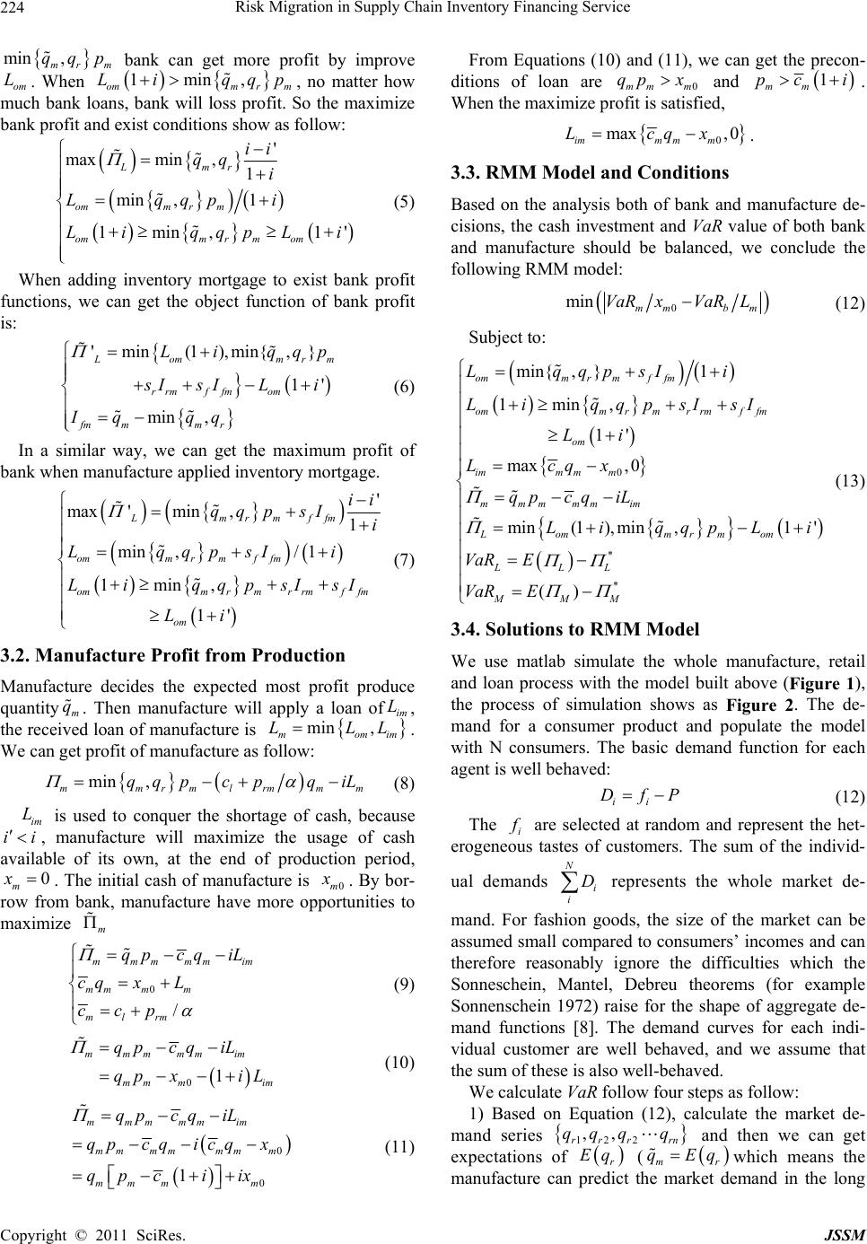
Calculate VaR of both manufacture and bank, then
standardize VaRto [0,1], then we can get

LL L M
VaR VaR VaR   basing on Equation (1) and
(2). Get
M

by 1
M
L

  , Table 1 shows the typical
data results of several experiments in computer simula-
tion when 01000
m
x、0.10i and '0.06i. With
different initial variables, the bank Va R will decrease
when adopt inventory mortgage, the potential profit is
growing. For the manufacture, after use inventory mort-
gage, VaR is larger than before. The potential income is
growing because bank can offer more loans which reduce
the manufacture shortage of cash, so the manufacture can
produce more to maximum profit.
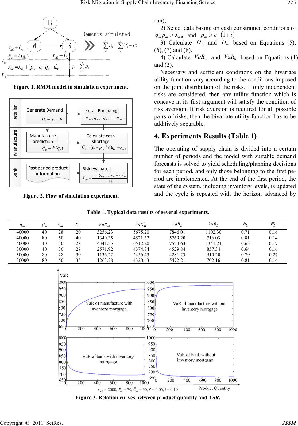
When the manufacture satisfies 0mm m
qp x and

1
mm
pc i
, accompany with market demand in-
creasing, the VaR of bank decrease because manufac-
ture’s capability of making profit. If using inventory
mortgage, the VaR value for manufacture is increasing
because more cash are put in producing and inven-
tory(Figure 3).
5. Conclusions
We discussed manufacture and retail supply chain struc-
ture which both facing cash-constrain and a bank that
finances the manufacturer. Supply chain inventory mort-
gage must satisfy preconditions of 0mm m
qp x and

1
mm
pc i, that is member of supply chain will use
self-owned capital before using inventory mortgage, and
the cost of loan must less than the profit rate. In inven-
tory mortgage, both bank and manufacture are benefit
because the risk migration. After migration of risk, it is
more compatible with the information shared between
supply chain member and bank. For supply chain mem-
bers, they have more market information than bank in
production operate process, after sharing inventory in-
formation with bank, this reduce the bank shortage in-
formation. So the migration of risk can help optimize the
whole supply chain and bank.
REFERENCES
[1] J. L. Cavinato, “Identifying Interfirm Total Cost Advan-
tages for Supply Chain Competitiveness,” International
Journal of Purchasing and Material Management, Vol.
27, No. 4, pp. 10-15.
[2] J. A. Buzacott, R. Q. Zhang, “Inventory Management
with Asset-Based Financing,” Management Science Vol.
50, No. 9, 2004, pp. 1274-1292.
doi:10.1287/mnsc.1040.0278
[3] T. Y. Choi and Y. Hong, “Unveiling the Structure of Sup-
ply Networks: Case Studies in Honda, Acura, and Dail-
mer Chrysler,” Journal of Operations Management, Vol.
20, No. 5, 2002, pp. 469-494.
doi:10.1016/S0272-6963(02)00025-6
[4] D. M. Lambert and M. C. Cooper, “Issues in Supply
Chain Management,” Industrial Marketing Management,
Vol. 29, No. 1, 2000, pp. 65-84.
doi:10.1016/S0019-8501(99)00113-3
[5] N. R. Srinivasa Raghavan and V. K. Mishra, “Short-Term
Financing in a Cash-Constrained Supply Chain,” Interna-
tional Journal of Production Economics, Vol. 11, No.14,
2009.
[6] D. Backus and J. Wright, “Cracking the conundrum,”
Brookings Papers on Economic Activity, Vol. 38, 2007,
pp. 293-329.
[7] P. Jorion, “Value at Risk: The New Benchmark for Con-
trolling Market Risk,” Irwin, Chicago, 1997.
[8] H. Sonnenschein, “Market Excess Demand Functions,”
Econometrica, Vol. 40, 1972, pp. 549-563.
doi:10.2307/1913184