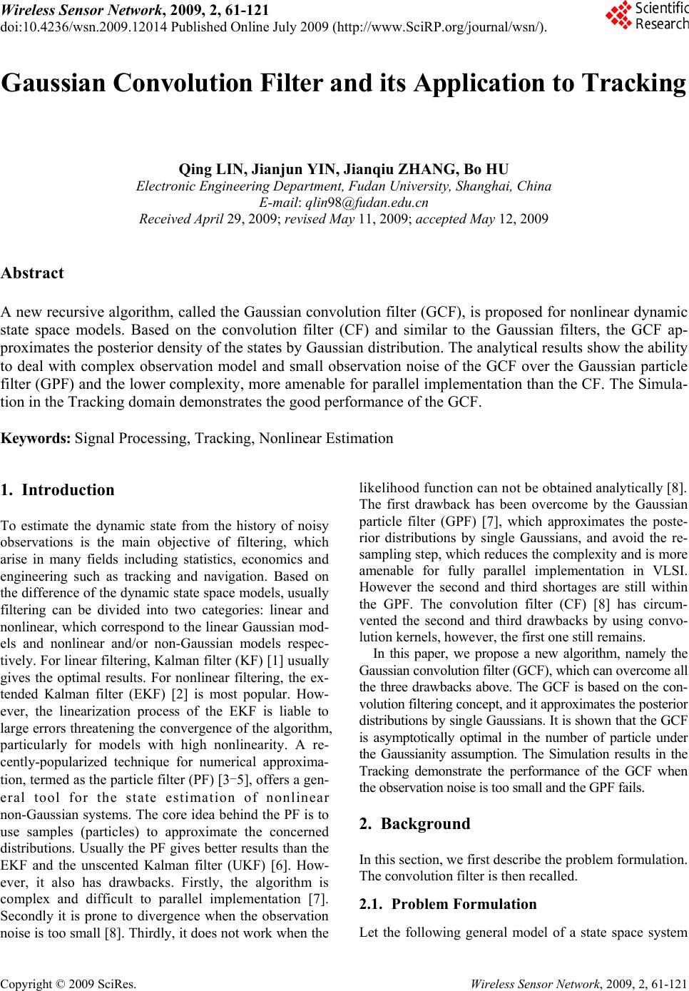Wireless Sensor Network, 2009, 2, 61-121
doi:10.4236/wsn.2009.12014 Published Online July 2009 (h ttp://www.SciRP.org/journal/wsn/).
Copyright © 2009 SciRes. Wireless Sensor Network, 2009, 2, 61-121
Gaussian Convolution Filter and its Application to Tracking
Qing LIN, Jianjun YIN, Jianqiu ZHANG, Bo HU
Electronic Engineering Department, Fudan University, Shanghai, China
Received April 29, 2009; revised May 11, 2009; accepted May 12, 2009
Abstract
A new recursive algorithm, called the Gaussian convolution filter (GCF), is proposed for nonlinear dynamic
state space models. Based on the convolution filter (CF) and similar to the Gaussian filters, the GCF ap-
proximates the posterior density of the states by Gaussian distribution. The analytical results show the ability
to deal with complex observation model and small observation noise of the GCF over the Gaussian particle
filter (GPF) and the lower complexity, more amenable for parallel implementation than the CF. The Simula-
tion in the Tracking domain demonstrates the good performance of the GCF.
Keywords: Signal Processing, Tracking, Nonlinear Estimation
1. Introduction
To estimate the dynamic state from the history of noisy
observations is the main objective of filtering, which
arise in many fields including statistics, economics and
engineering such as tracking and navigation. Based on
the difference of the dynamic state space models, usually
filtering can be divided into two categories: linear and
nonlinear, which correspond to the linear Gaussian mod-
els and nonlinear and/or non-Gaussian models respec-
tively. For linear filtering, Kalman filter (KF) [1] usu ally
gives the optimal results. For nonlinear filtering, the ex-
tended Kalman filter (EKF) [2] is most popular. How-
ever, the linearization process of the EKF is liable to
large errors threatening the convergence of the algorithm,
particularly for models with high nonlinearity. A re-
cently-popularized technique for numerical approxima-
tion, termed as the particle filter (PF) [3-5], offers a gen-
eral tool for the state estimation of nonlinear
non-Gaussian systems. The core idea behind the PF is to
use samples (particles) to approximate the concerned
distributions. Usually the PF giv es better results than the
EKF and the unscented Kalman filter (UKF) [6]. How-
ever, it also has drawbacks. Firstly, the algorithm is
complex and difficult to parallel implementation [7].
Secondly it is prone to divergence when the observation
noise is too small [8]. Thirdly, it d oes not work when th e
likelihood function can not be obtained analytically [8].
The first drawback has been overcome by the Gaussian
particle filter (GPF) [7], which approximates the poste-
rior distributions by single Gaussians, and avoid the re-
sampling step, which reduces the complexity and is more
amenable for fully parallel implementation in VLSI.
However the second and third shortages are still within
the GPF. The convolution filter (CF) [8] has circum-
vented the second and third drawbacks by using convo-
lution kernels, however, the first one still remains.
In this paper, we propose a new algorithm, namely the
Gaussian convolution filter (GCF), which can overcome all
the three drawbacks above. The GCF is based on the con-
volution filtering concept, and it approximates the posterior
distributions by single Gaussians. It is shown that the GCF
is asymptotically optimal in the number of particle under
the Gaussianity assumption. The Simulation results in the
Tracking demonstrate the performance of the GCF when
the observation noise is too small and the GPF fails.
2. Background
In this section, we first de scribe the problem formulation.
The convolution filter is then recalled.
2.1. Problem Formulation
Let the following general model of a state space system

Q. LIN ET AL.91
Copyright © 2009 SciRes. Wireless Sensor Network, 2009, 2, 61-121
)
be considered [3]:
1
(,
tttt
xfx


 (1)
(,)
tttt
yhx

 (2)
where t and t

denote the known independent process
and measurement noise respectively, {xt} the state of the
system complying with the Markov process, {yt} the
measurements of the system, and both ft and ht are
known nonlinear or linear functions. Again, let

1
,,

1
,
ttt

t
X
xxYyy
1
, and p(x0|x-1) = p(x0) be
the initial density. Here, the purpose is supposed to esti-
mate the posterior probability density function (pdf)
p(xt|Yt) by the Bayes recursion
 
1111ttttt tt
px|Ypx|xpx |Ydx

 (3)
  




ttttttttttt dx|Yxp|xyp|Yxp|xyp|Yxp 11 (4)
2.2. The Convolution Filter
Usually in PF scheme, the weight of each particle is
given by the likelihood function. The observations thus
operate the filter through the likeliho od function which is
assumed to exist and to be known. This assumption is
rather restricting in practice. Moreover it rules out the
non-noisy case and will also cause trouble when the ob-
servation noise is too small and also when the noise is
non-additive as in the general system (1) and (2). These
drawbacks can be circumvented by using convolution
kernels to weight the particles in the CF [8]. We can ap-
proximate the weights consistently by simulating the
observations, and use this approximation in place of the
true function in the PF, i.e.
 



|
ii
z
ttthnt
wpyx Kyy

i
t
(5)
where denote particle weights,

i
t
w
z
hn
K
is Par-
zen-Rosenblatt kernel of appropriate dimensions (A Par-
zen-Rosenblatt kernel is a bound ed positive and symmet-
ric function for which , where 1Kd  


is the
Lebesgue measure, and

lim 0
d
xKx as x,
where d is the dimension of variable y and  denotes
the squared norm), hn is called the kernel bandwidth, and


ˆi
t
y
are the samples from observation. Then we can get
the estimation as

 



11
ˆ |n
ii
x
ttt hnttt
ii
pxYwKxxw



n
i
(6)
A brief description of the resampled CF (RCF) is
given in Table 1.
Table 1. The RCF algorithm.
For 0t

Given p0 be the probability density of the initial state distribu-
tion
For 1t
(1) resample:


11
1~
n
i
tt
i
x
p



(2) evolving:
 
1
~(,),~( ,)
iiii
ttt ttt
xfxyhx


, 1,,in
(3) estimation:








1
1
|
nii
yx
hntthn tt
i
ttt ni
y
hn tt
i
K
yyKxx
pxY
Kyy





.
3. The Gaussian Convolution Filter
In this section, we present the main results of the paper,
the GCF recursion. The main idea behind the GCF is to
estimate the posterior distributions by CF, and then ap-
proximate them by Gaussians.
3.1. The Measurement Update
Assume the density of prediction is approximated by a
Gaussian [7], i.e.,



1;, tt ttt
px|Y x 



 (7)
where


;,x   denotes the Gaussian distribution
with the mean

and covariance . Take (7) as the
importance density and get samples from it, i.e.,





~;,,1,,
i
tttt
x
xi  N (8)
Obtain the observations




~( ,),1,,
ii
ttt
y
hx iN (9)
and the particle weights
 




ˆ|
ii
z
ttthnt
wpyx Kyy

i
t
(10)
By substituting (7) into (4) we get





;,
tt tttttt
px|Ym py|xx 


 (11)
where

 
1
1
ttttt
mpy|xpx|Yd

t x (12)
We approximate (11) by a Gaussian, i.e.,


;,
tt ttt
px|Y x 


 (13)
where
 
 




11
1
NN
ii i
tttt
ii
T
Nii ii
tttttt t
i
wx w
wx xw





 

 (14)

Q. LIN ET AL.
92
Copyright © 2009 SciRes. Wireless Sensor Network, 2009, 2, 61-121
where T
A
denotes the transpose of matrix A. We now
give the corollary to verify the convergence of the algo-
rithm above. Let us note that the form of corollary here is
similar to that in GPF [7], however the difference is that
the one here is based on the CF.
Corollary 1: Assume that at time t, the prediction dis-
tribution is Gaussian, i.e.


1;, tt ttt
px|Y x 
 .
The GCF measurement updates the filtering distribution
by the algorithm above. Then, t

computed in (14)
converges to the MMSE estimate of xt almost surely as
, and the MMSE estimate given by t in (14)
converges to the true MMSE estimate almost surely as
.
N
N

Proof: 1) mean

 

 





 
 
 
 
 


1
1
1
11
~| 1
1
1
1
1
1
ˆ|
ˆ|ˆ|
ˆ||
ˆ||
||
||
||
|
||
i
ttt
Nii
Nii
ttt
tt i
i
ttt NN
ii
ttt
ii
xpxY ttttt t
ttttt
ttttt t
ttttt
ttttt t
tt
ttttt
x
py x
xw
Ex Y
wpy
xpyxp xYdx
pyxpx Ydx
xpyxp xYdx
pyxpxYdx
xpyxp xYdx
pyY
xp xYdxE xY











 














t
x
.
(15)
2) covariance

























 
 
    
1
1
1
1
1
~| 1
1
ˆˆˆ
|||
ˆ|
ˆ|
||
ˆ||
ˆ||
||||
i
ttt
T
tttttttt
T
Nii i
ttttt
i
Ni
t
i
T
Nii i
tttt tt
i
Ni
tt
i
T
tttttt
xpxY
tttt t
tttt t
T
tttttt ttt
ExEx YxEx YY
xxw
w
xx pyx
py x
xExY xExY
pyxpx Ydx
pyxpx Ydx
xExY xExYpyxpx









 
















 




 






 



1
1
1
1
||
||||
|
|||
|||
tt
tttt t
T
t tttttttttt
tt
T
t tttttttt
T
ttttttt
Ydx
pyxpx Ydx
x
Ex YxEx YpyxpxYdx
py Y
xExY xExYpxYdx
ExExYxExYY






 
 




(16)
3.2. The Time Update
By substituting (13) to (3) we have



 
11tttt tt
px |Ypx|xpx|Ydx

t


 
1;, ttttt t
px |xxdx 

 (17)
Draw samples




~;,,1,,
i
t ttt
x
xi  N (18)
and then a Monte Carlo approximation of the predictive
distribution is given by



11
1
1Ni
tt tt
i
px |Ypx |x
N




(19)
Obtain samples at time t+1 from the process model by




11
~(,
i
ttt
xfx
 )
i
(20 )
from which the mean and covariance of are
computed as

1tt
px |Y






11
1
1111
1
1
1
Ni
tt
i
Nii
tttt
i
x
M
xx
1
t
M







 


(21)
Recall that the prediction distribution is approximated
as a Gaussian, we have

 
1 111
;,
tt ttt
px |Yx 

 


(22)
3.3. Summary of the GCF
We summarize the algorithm above in Table 2.
The GCF does away with the need of resampling step,
this means that the GCF is more amenable for fully paral-
lel implementation in VLSI than the CF. Moreover, be-
cause of the use of convolution kernels the GCF can deal
with scenarios that the observation noise is too small or
the likelihood function can not be obtained analytically.
4. Tracking Simulation Results
An example: Consider the problem of tracking a maneu-
vering target [9], who se position and velocity at instant t
are given by a continuous random vector x2t ∈ R
n-1,
and where the maneuver/regime of the target is repre-
sented by the discrete random variable x1k ∈ R. The
state to be estimated is xt ={x1t ; x2t}. The model is as
follows: X2t = Fx2t-1 + Bx1t + wt ;
Zt = Cx2t + et

Q. LIN ET AL.93
Copyright © 2009 SciRes. Wireless Sensor Network, 2009, 2, 61-121
Table 2. The GCF algorithm.
For 0t
Given  
0 000
;,px x   
For 1t
(1) Time update
(i) Draw samples from posterior density


1111
~;,,1,,
i
tttt
x
xi 

N
(ii) Draw samples from the process model
 
1
~( ,),1,,
ii
ttt
x
fx iN

(iii) Compute the mean and covariance





1
1
1
1
1
Ni
tt
i
T
Nii
tttt
i
x
M
xx
M

t





 


(2) Measurement update
(i) Draw samples from importance de n si t y


~;,,1,,
i
tttt
x
xi  N
(ii) Draw samples from the observation model
 
~( ,)
ii
ttt
yhx
(iii) Compute and normalized the weights
 

 
1
ˆ
ii
z
thntt
N
ii i
tt t
i
wKyy
ww w



(iv) Compute the mean and covariance
 
 



1
1
Nii
ttt
i
Nii i
t ttttt
i
wx
wx x






 


Additionally, given

2
111 11
(| )0.01,010
tttt t
px xxt~Ν, 

 .
t
w and are zero mean Gaussian noises, with co-
variance matrices Q and R. Since given X1t, the dynam-
ics of x2t are linear-Gaussian. In our model, we use
x2t=[xt yt xt’ yt’]T where (x; y) is the position of the target
in a cartesian plane. We take :
t
e
F=[1,0,0.3,0;0,1,0,0.3;0,0,1,0;0,0,0,1]T,
B=[1.25;-1.25;0.25;-0.25]T,
C=[1,0,0,0;0,1,0,0].
We use the simulation data as follows:
  
0 0.01,0;0,0.01,0,
t
t
ω~Ν,e~Ν,R 01
ˆ|
x

(20,
30, 0.5, 0.5)T where the measurement noise variance var-
ies during simulation. Both GCF and GPF are adopted in
the simulation. Figure 1 shows the absolute value of er-
rors of the state estimates given by the GPF (denoted by
asterisk-solid line) and GCF (denoted by dashed line)
respectively when the observation noise variance R=5. In
this case both the GPF and the GCF works well, also
shown in Table 3. However, when R is reduced, e.g.
R=0.1, the GPF diverges while the proposed GCF still
works well, as shown in Table 3, where

means the
divergence of the results as shown in [8], and the RMSE
Figure 1. Absolute value of estimated error (R=5).
Table 3. Detailed simulation results.
meth-
ods Rx position RMSE y position RMSE x velocity RMSE y velocity RMSE
108.6917279.132639 43.681761 42.659641
1 0.936217 0.898894 4.448537 5.993423
GPF 0.1




108.777454 9.123733 46.752717 47.554381
1 0.951737 0.901504 3.882222 5.185661
GCF 0.10.189300 0.198540 1.274176 1.247551
is calculated according to

2
1
ˆ
t
ii
i
x
xN


,
where ˆi
x
and i
x
are the estimated and true values
respectively, N denotes the total estimation times.
5. Conclusions
The proposed Gaussian convolution filter (GCF) over-
comes the drawbacks of the existing GPF, which is lim-
ited in the applications to scenarios that have non-noisy
or near non-noisy observations or lack the knowledge of
the likelihood function. Moreover the parallelizability of
the GCF and the absence of resampling step makes it
more convenient for VLSI implementation and, hence,
feasible for practical real-time applications than the ex-
isting CF. Simulation results are also presented to dem-
onstrate the performance of the GCF when the observa-
tion noise is small and the GPF fails.
6. References
[1] R. E. Kalman, “A new approach to linear filtering and
prediction problems,” Transactions of the ASME–Journal

Q. LIN ET AL.
94
Copyright © 2009 SciRes. Wireless Sensor Network, 2009, 2, 61-121
of Basic Engineering, Vol. 82-D, pp. 35–45, 1960.
[2] M. K. Steven, “Fundamentals of statistical signal process-
ing,” PTR Prentice-Hall, Englewood Cliffs, N.J., 1993.
[3] N. J. Gordon, D. J. Salmond, and A. F. M. Smith, “Novel
approach to nonlinear/non-Gaussian Bayesian state esti-
mation,” IEE Proceedings-F, Vol. 140, No. 2, pp. 107–113,
1993.
[4] A. Doucet, F. Nando, and N. J. Gordon, “Sequential
Monte Carlo in practice,” Springer, New York, 2001.
[5] T. Schon, F. Gustafsson, and P. J. Nordlund, “Marginal-
ized particle filters for mixed linear/nonlinear state-space
models,” IEEE Transactions on Signal Processing 2005,
Vol. 53, No. 7, pp. 2279–2289.
[6] J. J. Simon and K. U. Jeffrey, “Unscented filtering and
nonlinear estimation,” Proceedings of the IEEE, Vol. 92,
No. 3, pp. 401–422, 2004.
[7] J. H. Kotecha and P. M. Djuric, “Gaussian particle filter-
ing,” IEEE Transactions on Signal Processing, Vol. 51,
No. 10, pp. 2592–2601, 2003.
[8] V. Rossi and J.-P. Vila, “Nonlinear filter in discreet time:
A particle convolution approach,” Biostatic Group of
Monetepellier, Technical Report 04-03, 2004.
http://vrossi.free.fr/recherche.html.
[9] F. Mustiere, M. Bolic, and M. Bouchard, “A modified
Rao-blackwellised particle filter[C],” IEEE International
Conference on Acoustics, Speech and Signal Processing
(ICASSP) 2006, Toulouse, France, Vol. 3, pp. 21–24,
May 2006.