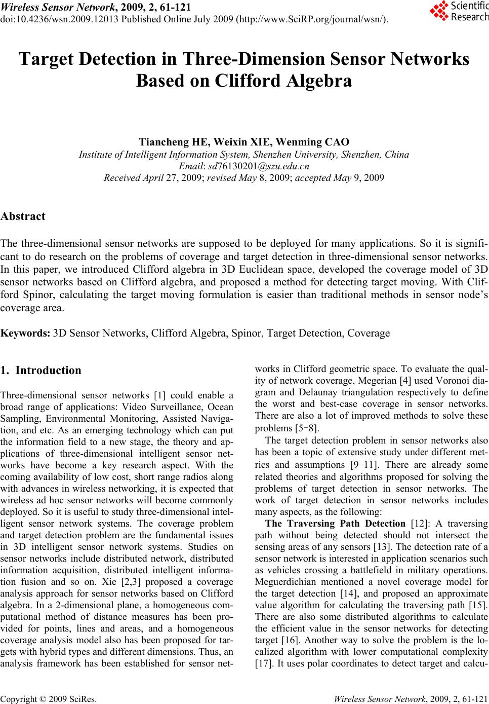Wireless Sensor Network, 2009, 2, 61-121
doi:10.4236/wsn.2009.12013 Published Online July 2009 (h ttp://www.SciRP.org/journal/wsn/).
Copyright © 2009 SciRes. Wireless Sensor Network, 2009, 2, 61-121
Target Detection in Three-Dimension Sensor Networks
Based on Clifford Algebra
Tiancheng HE, Weixin XIE, Wenming CAO
Institute of Intelligent Information System, Shenzhen University, Shenzhen, Ch ina
Received April 27, 2009; revised May 8, 2009; accepted May 9, 2009
Abstract
The three-dimensional sensor networks are supposed to be deployed for many applications. So it is signifi-
cant to do research on the problems of coverage and target detection in three-dimensional sensor networks.
In this paper, we introduced Clifford algebra in 3D Euclidean space, developed the coverage model of 3D
sensor networks based on Clifford algebra, and proposed a method for detecting target moving. With Clif-
ford Spinor, calculating the target moving formulation is easier than traditional methods in sensor node’s
coverage area.
Keywords: 3D Sensor Networks, Clifford Algebra, Spinor, Target Detection, Coverage
1. Introduction
Three-dimensional sensor networks [1] could enable a
broad range of applications: Video Surveillance, Ocean
Sampling, Environmental Monitoring, Assisted Naviga-
tion, and etc. As an emerging technology which can put
the information field to a new stage, the theory and ap-
plications of three-dimensional intelligent sensor net-
works have become a key research aspect. With the
coming availability of low cost, short range radios along
with advances in wireless networking, it is expected that
wireless ad hoc sensor networks will become commonly
deployed. So it is useful to study three-dimensional intel-
ligent sensor network systems. The coverage problem
and target detection problem are the fundamental issues
in 3D intelligent sensor network systems. Studies on
sensor networks include distributed network, distributed
information acquisition, distributed intelligent informa-
tion fusion and so on. Xie [2,3] proposed a coverage
analysis approach for sensor networks based on Clifford
algebra. In a 2-dimensional plane, a homogeneous com-
putational method of distance measures has been pro-
vided for points, lines and areas, and a homogeneous
coverage analysis model also has been proposed for tar-
gets with hybrid types and different dimensions. Thus, an
analysis framework has been established for sensor net-
works in Clifford geometric space. To evaluate the qual-
ity of network coverage, Megerian [4] used Voronoi dia-
gram and Delaunay triangulation respectively to define
the worst and best-case coverage in sensor networks.
There are also a lot of improved methods to solve these
problems [5-8].
The target detection problem in sensor networks also
has been a topic of extensive study under different met-
rics and assumptions [9-11]. There are already some
related theories and algorithms proposed for solving the
problems of target detection in sensor networks. The
work of target detection in sensor networks includes
many aspects, as the following:
The Traversing Path Detection [12]: A traversing
path without being detected should not intersect the
sensing areas of any sensors [13]. The detection rate of a
sensor network is interested in applicatio n scenarios such
as vehicles crossing a battlefield in military operations.
Meguerdichian mentioned a novel coverage model for
the target detection [14], and proposed an approximate
value algorithm for calculating the traversing path [15].
There are also some distributed algorithms to calculate
the efficient value in the sensor networks for detecting
target [16]. Another way to solve the problem is the lo-
calized algorithm with lower computational complexity
[17]. It uses polar coordinates to detect target and calcu-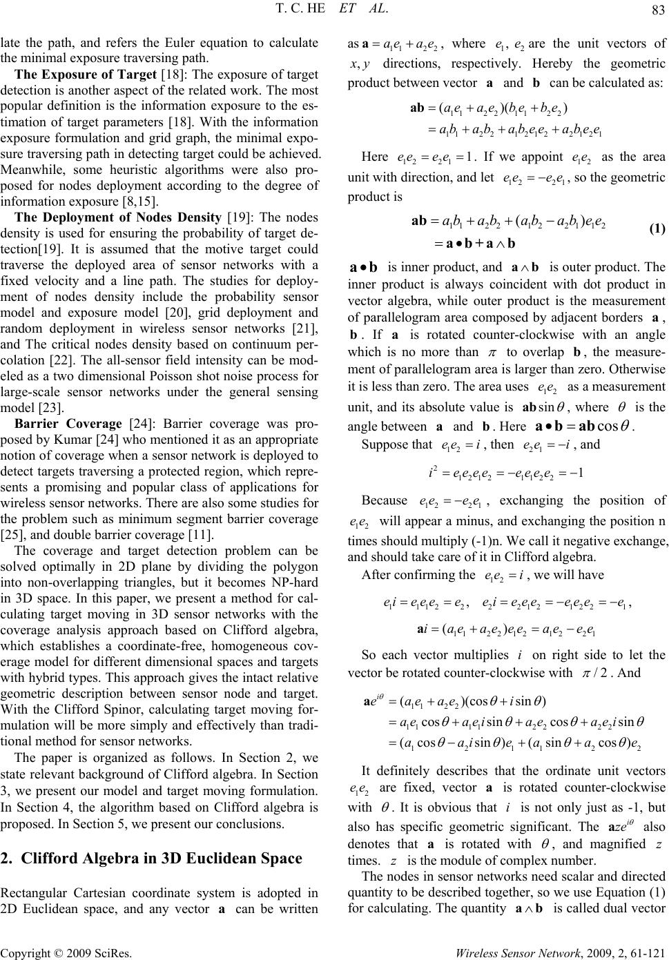

T. C. HE ET AL.
83
late the path, and refers the Euler equation to calculate
the minimal exposure traversing path.
The Exposure of Target [18]: The exposure of target
detection is another aspect of the related work. The most
popular definition is the information exposure to the es-
timation of target parameters [18]. With the information
exposure formulation and grid graph, the minimal expo-
sure traversing path in detecting target could be achieved.
Meanwhile, some heuristic algorithms were also pro-
posed for nodes deployment according to the degree of
information exposure [8,15].
The Deployment of Nodes Density [19]: The nodes
density is used for ensuring the probability of target de-
tection[19]. It is assumed that the motive target could
traverse the deployed area of sensor networks with a
fixed velocity and a line path. The studies for deploy-
ment of nodes density include the probability sensor
model and exposure model [20], grid deployment and
random deployment in wireless sensor networks [21],
and The critical nodes density based on continuum per-
colation [22]. The all-sensor field intensity can be mod-
eled as a two dimensional Poisson shot noise process for
large-scale sensor networks under the general sensing
model [23].
Barrier Coverage [24]: Barrier coverage was pro-
posed by Kumar [24] who mentioned it as an appropriate
notion of coverage when a sensor network is deployed to
detect targets traversing a protected region, which repre-
sents a promising and popular class of applications for
wireless sensor networks. There are also some studies for
the problem such as minimum segment barrier coverage
[25], and double barrier coverage [11].
The coverage and target detection problem can be
solved optimally in 2D plane by dividing the polygon
into non-overlapping triangles, but it becomes NP-hard
in 3D space. In this paper, we present a method for cal-
culating target moving in 3D sensor networks with the
coverage analysis approach based on Clifford algebra,
which establishes a coordinate-free, homogeneous cov-
erage model for different dimensional spaces and targets
with hybrid types. This approach g ives the intact relative
geometric description between sensor node and target.
With the Clifford Spinor, calculating target moving for-
mulation will be more simply and effectively than tradi-
tional method for sensor networks.
The paper is organized as follows. In Section 2, we
state relevant background of Clifford algebra. In Section
3, we present our model and target moving formulation.
In Section 4, the algorithm based on Clifford algebra is
proposed. In Section 5, we present our conclusions.
2. Clifford Algebra in 3D Euclidean Space
Rectangular Cartesian coordinate system is adopted in
2D Euclidean space, and any vector can be written
as
a
112 2
ae ae

a
,
, where are the unit vectors of
12
,ee
x
y
ab
12 2
ee e
directions, respectively. Hereby the geometric
product bet we en vector and can be calculated as: a
2 11
2 12
()e be
ab
b
12
(b
ee
112 2
11 2121
)ae e
ab aabee
 
 
2
2
a
b
Here 11e

. If we appoint as the area
unit with direction, and let , so the geometric
product is
12
ee
112
ee
2 21
b a
2
ee
2
b
1121 12
(abab ee a

 )

a b
ab
ab+ (1)

ab
a
is inner product, and is outer product. The
inner product is always coincident with dot product in
vector algebra, while outer product is the measurement
of parallelogram area composed by adjacent borders ,
. If is rotated counter-clockwise with an angle
which is no more than
ab
a
b

to overlap b, the measure-
ment of parallelogram area is larger than zero. Otherwise
it is less than zero. The area uses as a measurement
unit, and its absolute value is
12
ee
sin

ab , where

is the
angle between and b. Here acos

ab ab.
Suppose that 12
eei

, then , and
21
ee
12
i
2
i12 21eee e
12
e1 eee


Because 12
ee 2 ee
1

, exchanging the position of
will appear a minus, and exch anging the position n
times should multiply (-1)n. We call it negative exchange,
and should take care of it in Clifford algebra.
12
ee
111
eieee
After confirming the , we will have
12
ee i
2 2
i ee
222 122
,eeee e
1
e1 e

 
2 212
()aeee
,
111221
iae aeee


i
a
So each vector multiplies on right side to let the
vector be rotated counter-clockwise with /2

. And
11
11
(
cos
(cos
i
eae
ae

2 2
1 22
12 12
)(cos
cos sin
sincos )
ae
ae aei
aa aa
1s
sin
i22
1
)
e

2
e
sin
in
) (
i
a
ie



 
 

a
12
ee



It definitely describes that the ordinate unit vectors
are fixed, vector is rotated counter-clockwise
with
a

. It is obvious that is not only just as -1, but
also has specific geometric significant. The
i
i
ze

a also
denotes that is rotated with a

, and magnified
times. is the module of complex number. z z
The nodes in sensor networks need scalar and directed
quantity to be described together, so we use Equation (1)
for calculating. The quantity is called dual vector
ab
Copyright © 2009 SciRes. Wireless Sensor Network, 2009, 2, 61-121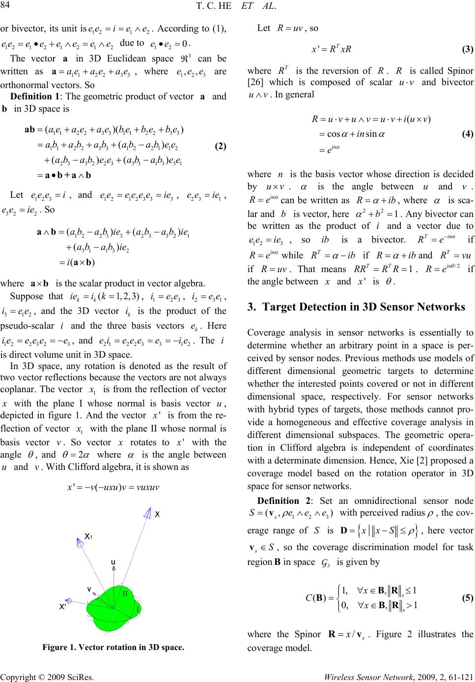

T. C. HE ET AL.
84
Copyright © 2009 SciRes. Wireless Sensor Network, 2009, 2, 61-121
)
or bivector, its unit is. According to (1),
due to .
121 2
eei ee 
1 2
ee
2 23 3
ae ae
233112
2 3312
32 2331
()(
(
) (
aebebe
ababab
ab eeab
 
 

b
12 1233
ee eeee
121 212
eeeeee
a
11
aea
b
11 2
11 2
23
(
ae ae
ab ab
ab




ab
ab+a
123
eee i
12
0ee
3

ee
2 33
21 12
13 31
)
)
be
ee
abee


3
ie
The vector in 3D Euclidean space can be
written as , where are
orthonormal vectors. So 123
,,e
Definition 1: The geometric product of vector and
in 3D space is a
(2)
Let , and

, 23 1 ee ie

,
. So
32 2
ee ie
12
(
(
ab
i


ab
ab
21323
3113 2
()
)
)
ab ieab
abab ie
 

ab
(1,2,3)
kk
i k
32 1
(ab ie
123
iee
)
1
where is the scalar product in vector algebra.
Suppose that ie , , 23
iee

,
, and the 3D vector is the product of the
pseudo-scalar and the three basis vectors . Here
, and . The
is direct volume unit in 3D space.
312
iee
i
12 2323
ie eeee
k
i
212 2 3
eieee
1
k
e
i
312
e ie
In 3D space, any rotation is denoted as the result of
two vector reflections because the vectors are not always
coplanar. The vector
x
is from the reflection of vector
x
with the plane I whose normal is basis vector ,
depicted in figure 1. And the vector u '
x
is from the re-
flection of vector 1
x
with the plane II whose normal is
basis vector . So vector v
x
rotates to '
x
with the
angle

, and 2

  where

is the angle between
and v. With Clifford algebra, it is shown as u
'()
x
vuxu vvuxuv 
Figure 1. Vector rotation in 3D space.
Let Ruv

, so
'T
x
RxR (3)
where is the reversion of . is called Spinor
[26] which is composed of scalar u and bivector
T
RRRv
uv

. In general
()
cossin
in
Ruvuvuviuv
in
e



 


(4)
where is the basis vector whose direction is decided
by n vu

.

is the angle between and . uv
in
Re

can be written as Rib

 , where

is sca-
lar and is vector, here . Any bivector can
be written as the product of i and a vector due to
b
3
ie
22
1b  
12
ee

, so ib is a bivector. T
Re
in


 if
in
Re

while T Ri  b

 if Rib

and T Rvu

if Ruv

. That means . if
the angle between 1
TT
RRR R /2in

Re
x
and '
x
is

.
3. Target Detection in 3D Sensor Networks
Coverage analysis in sensor networks is essentially to
determine whether an arbitrary point in a space is per-
ceived by sensor nodes. Previous methods use models of
different dimensional geometric targets to determine
whether the interested points covered or not in different
dimensional space, respectively. For sensor networks
with hybrid types of targets, those methods cannot pro-
vide a homogeneous and effective coverage analysis in
different dimensional subspaces. The geometric opera-
tion in Clifford algebra is independent of coordinates
with a determinate dimension. Hen ce, Xie [2] proposed a
coverage model based on the rotation operator in 3D
space for sensor networks.
Definition 2: Set an omnidirectional sensor node
123
(, )
s
Seee


v with perceived radius

, the cov-
erage range of is S


|xxS

D, here vector
sS

v
B3 G
, so the coverage discrimination model for task
region in space is given by
1,, 1
() 0,, 1
x
Cx

 






BR
BBR
x
x
(5)
where the Spinor /
s
x

Rv
. Figure 2 illustrates the
coverage model.

T. C. HE ET AL.
85
Copyright © 2009 SciRes. Wireless Sensor Network, 2009, 2, 61-121
S
Vs
x
B
2
22
2
'()(
()()
()
()()
T
R Ribib
ibi b
ibib bb
ib ib b
ibibR


)

 
 
 
 
 

 
 
Here the exchange among vector

, pseudo-scalar
and
i

is positive, but is negative between

and vec-
tor .
b
With 2
'R

, consider 1
TTT
RRReRRR

 
, here
3
2
11 1
13
12
(cossin)
cossin
ie T
ReR eRee
eie
ee

 





(8)
Figure 2. Coverage model based on Clifford Spinor in 3D
space.
The relationship between sensor node and target is al-
ways depicted by Euler angle, and it would be illustrated
by Clifford algebra without coordinates. So the Clifford
algebra can present 3×3 Spinor matrix, and the angle
transformation is
And
1
12
12
12 3
(cos sin)
cossin
cossincossinsin
T
ie
Ree R
eee
ee e










 
(9)
333 333
/2/2/2/2 /2 /2
TTT
ieieieie ie ie
xRRRxRRR
eeexeee
 

  


R (6) So
33
11 23
12 3
122
13
(cossincossinsin )
cos()sincos()sinsin
coscoscossinsincoscos
sincossinsinsin
T
ie ie
fRe eeR
eee ee
eee
ee




 


 
 
 


Let , and is the new vector that is iso-
morphic with in new position after transformation.
e
k
fR
ek
kk
f

(10)
Theorem 1: The vector

which is perpendicular
with axis rotates to

, so
2
'T RR R

 R (7) Meanwhile
221 1
23
cos cos coscos sin sinsincos
sinsincossin
fee e
ee

 
 



(11)
Proof:

is perpendicular with vector b in R

ib

 whose direction is same as axis, so bb



bb bb
 
, that means the negative
exchange between vectors which are perpendicular with
each other. So 33 21
cossin cossinsinfe ee

 

 (12)
The Spinor matrix (
jkj k
Rfe)

 is
coscossin cossincossinsincoscossin sin
cos sin sinsincoscos coscossinsincos sin
sin sinsin coscos
jk
R



 
 



 




(13)
With the method of Clifford algebra, we can easily
calculate the 3×3 Spinor matrix of arbitrary angle

rotating around any vector . The element of this ma-
trix is n
circumstance can be written as .
Here
0
()
T
jkj k
RReRe 
0

denotes the vector of grade zero which is
scalar part, because the result will normally be
01 2 3

 
jk
R
 . We have known that the
established just is a simple scalar quantity, so we
don’t have to denote its vector of grade zero, where
(' )
j
kjk j
RfeReRe 
k
(14)
Generally, it is more suitable that the element under this

T. C. HE ET AL.
86
Copyright © 2009 SciRes. Wireless Sensor Network, 2009, 2, 61-121
j
)
2
()()
()()
Tjj
jj
jjj
ReRibe ib
ibeie b
eibeiebbeb




 
 
With
()2()2()2(
jj jjj
iebbeieb iiebeb

   
,
2
()(
2
jjj jj
jjj j
bebbeb ebbeb eb
bebbbee bbbebbe
 
 
)
j
j
Hence
22
()2()2
Tjjj
ReRbeebb eb   
,
And
22
)( )2)(
Tjjkj
(()2( )
jjjk
R
eRebebeb eeb 

 
where cos 2

 , sin 2 bn

,

is the angle, nis the
unit vector for rotating. (3.10) can be written as
cosin()(1coss)
j
kjkjkjk
nenRen

 

 
Here
(15)
j
k

is Kronecker symbol. When jk, 1
jk


,
otherwise 0
jk


. The second part in (15) is a general
vector operation wated by spe-
cific )
j k
enen
hich can be easily calcul
j,kbecause () (
kj
e e

 
2
 . For exam-
ple, j

, 3k

, and23 1 ee e, so ()n
j
ek e


11
enn

. Therefore, the second part is 1sinn

here
which can infer the other parts. The final result is
2
1123132
2
123223 1
2
312 3113
cos(1cos)(1cos )sin(1cos)sin
(1cos)sincos(1cos )(1cos)sin
(1 cos)sin(1 cos)sincos(1 cos)
jk
nnnnnnn
Rnnnnnn n
nnn nnnn



 
 

 

 


 


The conventional methods can also achieve this result,
but this method is straight and do not need the graph for
help. Hence the target moving can be detected in cover-
age area of sensor networks by Clifford algebra, as
shown in figure 3. If the target moves from
x
to '
x
,
that is
'T
x
RxR ax aR (1)
where
6
x
is the position of target.
Each element in (16) would be time fu
onction, so the target mving formulation is
'
x
xxaRR


(17)
Theorem 2: In (17), TT
x
RxR RxRR

can be cal-
culated by (18):
()
T
x
Rx   R
where
R
 (18)

is target’s angular velocity to sensor node.
Proof: Suppose that
1RRx 2



And
0
TT
RR RR



11
0
22
TT T
RRRR



1
,2
TT
RR 
T
Here 1
T
RR

,
ted as
()
TT
RR

.
i
 is bector, and can
be deno
iv


. So 2T RR
 orR 2T
iR  .
Thus
11
T T1
()
22 2
TTT TT
x
RxRRRxRRR RxxR RR R

and
xR RxR

1()(
2
TT
)
x
RxxRxRxRR
 R
Or
()(
2
TT
i
()
x
ix



 and ()
x
ix

  ,
)
x
Rx xRRx   R
 R
With
'[()]
T
x
RxxR  a

    (19)
The target moving formulation can further be denoted
as
'[()][()()]
x
xxx xxa 

 RR

 (20)

T. C. HE ET AL.
87
X' X
S
Figure 3. The target moving path de te cted by sensor node.
where
() ()()
11
'()()'
TT
iR xRRxRi
22
[()''()]
2
[()()]
2
()
()
TT
TTT
T
T
T
xR xRRxR
i
R
xR RR RxR
i
Rx xR
RxR
Rx R
 


  
 


 
 



R
 
And
()
TT TT
x
RxR RxRRxRRxR  R
 
 
.
Therefore,
'[2() ()]
T
x
Rxxx xRa  

 (21)
In the 3D space, the movement formulation of the tar-
ge
w
'
t m is
''mx g
 ,
here is the power of the target so
[
T2() ()]
R
mxxxxR mag  
 
[2() ()]'
TT
mxxxxRmaRRgRg   
  
[2() ()]T mxg mxxxRmaR   


We can achieve the movement formulation of the tar-
get in sensor networks, which will help us to analyze the
state of the detected target.
4.
otive target detection algor-
ithm based on Clifford Spinor. We assume that the mo-
or networks can be detected by some
n the range of these nodes also
Algorithm
With the movement formulation of the target in 3D sen-
sor netw orks, we pr opose a m
tive target in sens
nodes, and its positions i
can be calculated. Because the surveillance range of a
node is always small, the track of the target in the range
will be considered as a line approximately. Our algo-
rithm for tracking the motive target is following:
1) Detect the two vertexes of the track when the target
is in the range of node;
2) Use (17) or (20) to calculate the movement formu-
lation of the target;
3) Use the movement states of target to estimate the
direction and velocity so as to inform the next correlative
node turning on and starting to detect the target;
4) Collect all information from each node, and achieve
the track of the motive target in the sensor networks.
Figure 4 shows the motive target detection using
moving formulation calculated by Clifford Spinor in 3D
sensor networks, where (a) is the target’s actual path to
traverse sensor networks, and (b) is the target’s travers-
ing path achieved by moving formulation. The target
positions in sensor’s coverage area can be used to calcu-
late the moving formulation to get the traversing path in
this area. Connecting all of these paths which are
achieved from each node can get the target’s track in
sensor networks. It is helpful for target tracking and
forecasting.
(a)
(b)
Figure 4. Target dete ction in 3D se nsor networks.
Copyright © 2009 SciRes. Wireless Sensor Network, 2009, 2, 61-121

T. C. HE ET AL.
88
Copyright © 2009 SciRes. Wireless Sensor Network, 2009, 2, 61-121
100 200 300400500 600 700 800 9001000
0
5
10
15
20
25
30
35
40
45
Number of Sensor No des
Cpu T im e
Time C onsuming of Three Methods
Cliff ord Me thod
Pauli Method
Cartesian Method
[5] Figu hree
methods.
Figure 5 denotes the time consuming to calculate tar-
get moving formulation using Cartesian method, polar
coordinates method and Clifford method, respectively. It
is obvious that the time consuming using Clifford
method is lower than that of the other two methods
the number of sensor nodes increases. This is because the
Cartesian method should use the information of three
axes in 3D space and the polar coordinates me
would calculate three 3×3 Pauli matrices. The quantity of
calculation is decreased in Clifford method due to just
using Spinor equation to get the moving formulation
without axes information in 3D space.
lusions
ported by National Natural Science
on Clifford algebra,” Science
in China Series F-Information Sciences, Vol. 51, No. 5,
[3] W. X. Xie, T. C. He, and W. M. Cao, “Path analyses of
B.
Srivastava, “Worst and best-case coverage in sensor net-
ransactions on Mobile Computing, Vol. 4,
No. 1, pp. 84–92, 2005.
bedded Networked Sensor Sys-
babilistic
diagram,” Jour-
chnology, Vol. 23, No. 1, pp. 154–165, 2008.
i, J. Wu, M. Lu, and M. O. Pervaiz, “Maximum
l,
oc
sensor networks,” in IEEE INFOCOM, Vol. 3, pp.
1380–1387, 2001.
re 5. The comparison of time consuming among t
[6]
when
[7] A. D. Gupta, A. Bishnu, and I. Sengupta, “Optimisation
problems based on the maximal breach path measure for
wireless sensor network coverage,” ICDCIT, pp. 27–40,
2006.
thod [8] G. Veltri, Q. Huang, G. Qu, and M. Potkonjak, “Minimal
and maximal exposure path algorithms for wireless em-
bedded sensor networks,” Proceedings of the 1st Interna-
tional Conference on Em
5. Conc
In this paper, we developed the coverage model of 3D
sensor networks with the coverage analysis approach
based on Clifford algebra, which establishes a coordi-
nate-free, homogeneous coverage model for different
dimensional spaces and targets with hybrid types, and
proposed the method for detecting target moving. With
Clifford Spinor, calculating the target moving formula-
tion is easier than traditional methods in sensor node’s
coverage area. It is helpful to the research of coverage
analysis in sensor network s.
6. Acknowledgements
This research is sup
Foundation (No.60872126) and Guangdong Province
Natural Science Foundation (No.8151806001000002).
7. References
[1] C. Tian, W. Liu, J. Jin, Y. Wang, and Y. Mo, “Localiza-
tion and synchronization for 3D underwater acoustic
sensor network,” Proceedings of UIC 2007, pp. 622–631,
July 2007.
[2] W. X. Xie, W. M. Cao, a nd S. Meng, “Coverage analysi s
for sensor networks based
pp. 460–475, 2008.
sensor networks based on Clifford algebra,” Acta Elec-
tronica Sinica, Vol. 35, No. 12A, pp. 27–31, 2007.
[4] S. Megerian, F. Koushanfar, M. Potkonjak, M.
works,” IEEE T
X. Li, P. Wan, and O. Frieder, “Coverage problem in
wireless ad-hoc sensor networks,” IEEE Transactions on
Computers, Vol. 52, No. 6, pp. 753–763, 2003.
T. C. He, W. M. Cao, and W. X. Xie, “Research of
breach issue for sensor networks based on Clifford geo-
metrical algebra,” Chinese Journal of Scientific Instru-
ment, Vol. 28, No. 8, pp. 161–165, 2007.
tems (SenSys’03), Los Angels, CA, USA, pp. 40–50,
2003.
[9] L. Lazos, R. Poovendran, and J. A. Ritcey, “Pro
detection of mobile targets in heterogeneous sensor net-
works,” in Proceedings of IPSN’07, pp. 519–528, 2007.
[10] W. Z. Zhang, M. L. Li, and M. Y. Wu, “An al gorithm for
target traversing based on local Voronoi
nal of Software, Vol. 18, No, 5, pp. 1246–1253, 2007.
[11] C. D. Jiang and G. L. Chen, “Double barrier coverage in
dense sensor networks,” Journal of Computer Science
and Te
[12] M. Cardei, M. T. Thai, Y. Li, and W. Wu, “En-
ergy-efficient target coverage in wireless sensor net-
works,” Proceedings of IEEE INFOCOM’05, Miami, FL,
pp. 1976–1983, 2005.
[13] M. Carde
network lifetime in wireless sensor networks with ad-
justable sensing ranges,” Proceedings of IEEE Interna-
tional Conference on Wireless and Mobile Computing,
Networking and Communications (WiMob’05), Montrea
Canada, pp. 1–8, 2005.
[14] S. Meguerdichian, F. Koushanfar, M. Potkonjak, and M.
B. Srivastava, “Coverage problems in wireless ad-h

T. C. HE ET AL.
89
Copyright © 2009 SciRes. Wireless Sensor Network, 2009, 2, 61-121
ro-
discrete targets in wireless sensor
, 2002.
Srivastava, “Critical density thresh-
orst and best information exposure
997.
Mobile Ad-hoc and
l Conference on Robotics and
[15] S. Meguedrichian, S. Slijepcevic, V. Karayan, and M.
Potkonjak, “Localized algorithms in wireless ad-hoc
networks: Location discovery and sensor exposure,” P
ceedings of ACM MobiHoc’01, Long Beach, CA, USA,
pp. 106–116, 2001.
[16] M. Lu, J. Wu, M. Cardei, and M. Li, “Energy-efficient
connected coverage of
networks,” Proceedings of 2005 International Conference
on Computer Networks and Mobile Computing (ICCN-
MC’05), Zhangjiajie, China, pp. 1–10, 2005.
[17] X. Li, P. Wan, and O. Frieder, “Coverage in wireless
ad-hoc sensor networks,” Proceedings of IEEE Interna-
tional Conference on Communications (ICC’02), New
York, NY, USA, pp. 1–5
[18] S. Meguerdichian, F. Koushanfar, G. Qu, and M. Potkon-
jak, “Exposure in wireless ad hoc sensor networks,” Pro-
ceedings of ACM MobiCom’01, pp. 139–150, 2001.
[19] S. Adlakha and M.
olds for coverage in wireless sensor networks,” Proceed-
ings of IEEE Wireless Communications and Networking
Conference (WCNC’03), NewOrleans, Louisiana, USA,
pp. l6–20, 2003.
[20] B. Wang, et al., “W
paths in wireless sensor networks,” Proceedings of MSN
2005, pp. 52–62, December 2005.
[21] B. Liu and D. Towsley, “On the coverage and detectabil-
ity of large-scale wireless sensor networks,” Proceedings
of WiOpt’03: Modeling and Optimization in Mobile, Ad
Hoc and Wireless Networks, INRIA Sophia-Antipolis,
France, pp. 1–3, 2003.
[22] R. Meester and R. Roy, “Continuum percolation,” Bal-
letin of the American Mathematical Society, Vol. 34, No.
4, pp. 447–448, 1
[23] B. Liu and D. Towsley, “A study of the coverage of
large-scale sensor networks,” Proceedings of the 1st
IEEE International Conference on
Sensor Systems (MASS’04), Florida, USA, pp. 475–481,
2004.
[24] S. Kumar, T. Lai, and A. Arora, “Barrier coverage with
wireless sensors,” Wireless Network, Vol. 13, pp. 817–
834, 2007.
[25] S. Kloder and S. Hutchinson, “Barrier coverage for vari-
able bounded-range line-of-sight guards,” in Proceedings
of IEEE Internationa
Automation 2007, pp. 391–396, April 2007.
[26] J. O’Rourke, “Computational geometry: Column 15,”
International Journal of Computational Geometry and
Applications, Vol. 2, No. 2, pp. 215–217, 1992.