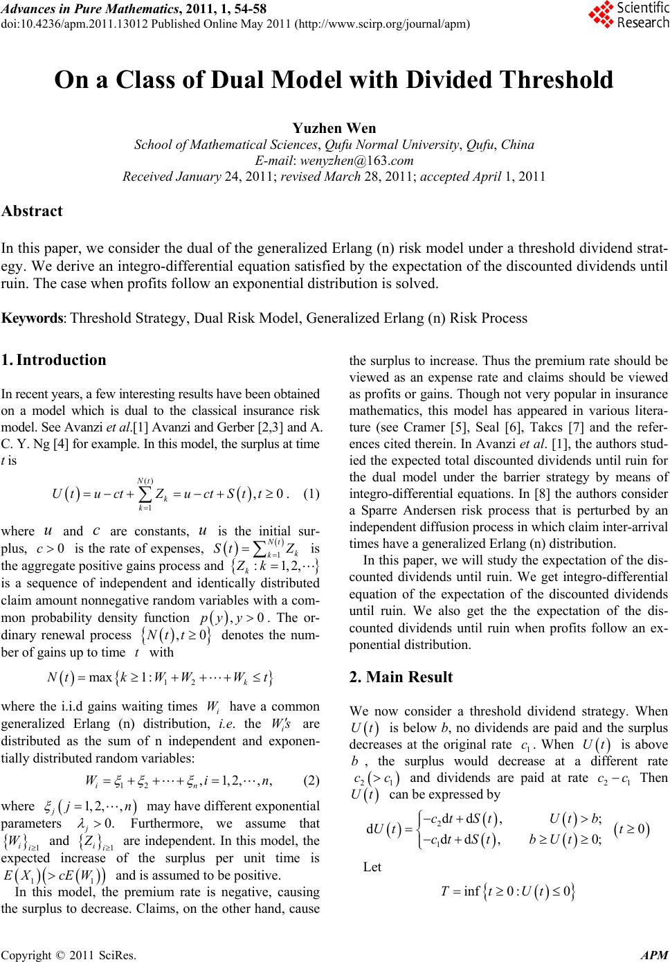
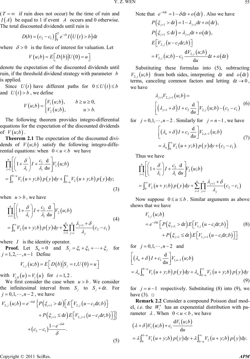
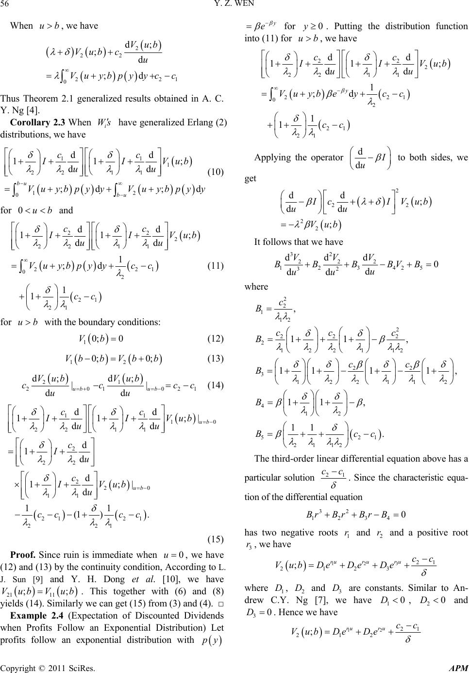
Advances in Pure Mathematics, 2011, 1, 54-58
doi:10.4236/apm.2011.13012 Published Online May 2011 (http://www.scirp.org/journal/apm)
On a Class of Dual Model with Divided Threshold
Yuzhen Wen
School of Mathemat i cal Sci ences, Qufu Normal University, Qufu, China
Received January 24, 2011; revised March 28, 2011; acce pted April 1, 2011
Abstract
In this paper, we consider the dual of the generalized Erlang (n) risk model under a threshold dividend strat-
egy. We derive an integro-differential equation satisfied by the expectation of the discounted dividends until
ruin. The case when profits follow an exponential distribution is solved.
Keywords: Threshold Strategy, Dual Risk Model, Generalized Erlang (n) Risk Process
1. Introduction
In recent years, a few interesting results have been obtained
on a model which is dual to the classical insurance risk
model. See Avanzi et al.[1] Avanzi and Gerber [2,3] and A.
C. Y. Ng [4] for example. In this model, the surplus at time
t is
 
()
1
,0
Nt
k
k
UtuctZuctSt t

  
. (1)
where u and c are constants, u is the initial sur-
plus, 0c is the rate of expenses,



1
Nt
k
k
St Z

 is
the aggregate positive gains process and


:1,2,
k
Zk
is a sequence of independent and identically distributed
claim amount nonnegative random variables with a com-
mon probability density function

,0py y. The or-
dinary renewal process
 
,0Nt t denotes the num-
ber of gains up to time t with
 
12
max 1:k NtkW WWt
where the i.i.d gains waiting times i W have a common
generalized Erlang (n) distribution, i.e. the i
Ws

are
distributed as the sum of n independent and exponen-
tially distributed random variables:
12 ,1,2,,, in
Win

   (2)
where

1, 2,,
jjn
  may have different exponential
parameters 0.
j

 Furthermore, we assume that

1
ii
W and

1
ii
Z are independent. In this model, the
expected increase of the surplus per unit time is
  
11
EX cEW and is assumed to be positive.
In this model, the premium rate is negative, causing
the surplus to decrease. Claims, on the other hand, cause
the surplus to increase. Thus the premium rate should be
viewed as an expense rate and claims should be viewed
as profits or gains. Though not very popular in insurance
mathematics, this model has appeared in various litera-
ture (see Cramer [5], Seal [6], Takcs [7] and the refer-
ences cited therein. In Avanzi et al. [1], the authors stud-
ied the expected total discounted dividends until ruin for
the dual model under the barrier strategy by means of
integro-differential equations. In [8] the authors consider
a Sparre Andersen risk process that is perturbed by an
independent diffusion process in which claim inter-arrival
times have a generalized Erlang (n) distribution.
In this paper, we will study the expectation of the dis-
counted dividends until ruin. We get integro-differential
equation of the expectation of the discounted dividends
until ruin. We also get the the expectation of the dis-
counted dividends until ruin when profits follow an ex-
ponential distribution.
2. Main Result
We now consider a threshold dividend strategy. When


Ut is below b, no dividends are paid and the surplus
decreases at the original rate 1 c. When

Ut is above
b, the surplus would decrease at a different rate


21
cc and dividends are paid at rate 21 cc

Then


Ut can be expressed by



 
2
1
dd ,;
ddd ,0;
ct StUt b
Ut ctStb Ut

 








0t
Let



inf0 :0TtUt



Y. Z. WEN 55
(T if ruin does not occur) be the time of ruin and

I
A be equal to 1 if event
A
occurs and 0 otherwise.
The total discounted dividends until ruin is
  
21
0
() d
Tt
DbcceIUtbt
 
 

where 0

 is the force of interest for valuation. Let
 
;0Vub EDbUu



denote the expectation of the discounted dividends until
ruin, if the threshold dividend strategy with parameter b
is applied.
Since

Ut have different paths for


0Ut b
and

Ut b, we define
 

1
2
;, 0,
;;, .
Vubb u
Vub Vubub





The following theorem provides integro-differential
equations for the expectation of the discounted dividends
of

;Vub.
Theorem 2.1 The expectation of the discounted divi-
dends of

;Vub satisfy the following integro-diffe-
rential equations: when 0ub we have

 
1
1
1
12
0
d
1;
d
;d ;d;
n
iii
bu
bu
c
IVub
u
Vu ybpy yVu ybpy y








 



 


(3)
when ub, we have

 
2
2
1
1
221
01
d
1;
d
;d
n
iii
n nj
iji j
c
IVub
u
Vu ybpyycc










 




 



(4)
where
I
is the identity operator.
Proof. Let 00S and 12
j
j
S
 
 for
1, 2,,1jn Define
 
,;,0 ij j
Vub EDbS tUu



with
 
,0ii
VuVu for 1, 2 i.
We first consider the case when ub. We consider
the infinitesimal interval from
j
S to d.
j
St

For
0,1, ,2jn, we have
  





2,12, 2
12,12
21
;dd;
dd;
1.
dt
jjj
jj
dt
Vube PtEVuctb
PtEVuctb
e
cc










 




 




(5)
Note that

d1d d t
etot


 . Also we have






  
11
11
2, 2
2,
2, 2
d1dd,
ddd,
d;
d;
;dd
d
jj
jj
j
j
j
Pt tot
Pttot
EVuc tb
Vub
Vubc tot
u




 
 



 
Substituting these formulas into (5), subtracting


2, ; j
Vub from both sides, interpreting dt and


dot
terms, canceling common factors and letting d0t,
we have



 
12, 1
122,21
;
d;
d
jj
jj
Vub
I
cVubcc
u






 


(6)
for 0,1,,2jn

. Similarly for 1jn , we have
 

22,1
221
0
d;
d
;d .
nn
n
IcV ub
u
Vu ybpyycc








 

(7)
Thus we have

 
2
2
1
1
221
01
d
1;
d
;d
n
iii
n nj
iji j
c
IVub
u
Vu ybpyycc










 




 



Now suppose 0ub

. Similar arguments as above
shows that we have






1,
d
11,1
11,11
;
dd;
dd;
j
tjj
jj
Vub
eP tEVuctb
PtEVuctb











  


(8)
for 0,1,,2jn

 and
 
 
11,1
12
0
d;
d
;d ;d
nn
bu
nn
bu
IcVub
u
Vu ybpy yVu ybpy y









 

(9)
for 1jn

 respectively. Substituting (8) into (9), we
have (3). □
Remark 2.2 Consider a compound Poisson dual mod-
el, i.e. the i
W

has an exponential distribution with pa-
rameter

. When 0ub

, we have



 
1
11
12
0
d;
;d
;d ;d.
bu
bu
Vub
Vub cu
Vu ybpy yVu ybpy y





 


Y. Z. WEN 56
When ub, we have
 

2
22
221
0
d;
;d
;d
Vub
Vub cu
Vuybpyyc c




 

Thus Theorem 2.1 generalized results obtained in A. C.
Y. Ng [4].
Corolla ry 2.3 When i Ws
 have generalized Erlang (2)
distributions, we have

 
11
1
22 11
12
0
dd
11 ;
dd
;d ;d
bu
bu
cc
IIVub
uu
Vu ybpy yVu ybpy y

 



 
 
  

 

 

(10)
for 0ub and

 

22
2
22 11
221
0
2
21
21
dd
11 ;
dd
1
;d
1
1
cc
I
IVub
uu
Vuybpyyc c
cc

 





 
 
  

 

 

 


 (11)
for ub with the boundary conditions:

10; 0Vb (12)

12
0; 0;Vbb Vbb  (13)



21
201021
d; d;
||
dd
ub ub
Vub Vub
cccc
uu
 
 (14)


 
11
10
22 11
2
22
2
20
11
21 21
221
dd
11 ;|
dd
d
1d
d
1;|
d
11
(1 ).
ub
ub
cc
IIVub
uu
c
Iu
c
IVub
u
cc cc

 










 
 
  

 




 





 
 



 
(15)
Proof. Since ruin is immediate when 0u, we have
(12) and (13) by the continuity condition, According to L.
J. Sun [9] and Y. H. Dong et al. [10], we have
 
21 11
;;Vub Vub. This together with (6) and (8)
yields (14). Similarly we can get (15) from (3) and (4). □
Example 2.4 (Expectation of Discounted Dividends
when Profits Follow an Exponential Distribution) Let
profits follow an exponential distribution with


py
y
e



 for 0y. Putting the distribution function
into (11) for ub, we have

 

22
2
22 11
221
0
2
21
21
dd
11 ;
dd
1
;d
1
1
y
cc
I
IVub
uu
Vuybeycc
cc


 





 
 
  

 

 

 



Applying the operator d
d
I
u





to both sides, we
get
 

2
22
2
2
dd ;
dd
;
I
cIVub
uu
Vub


 



 

It follows that we have
32
222
123425
32
ddd 0
d
dd
VVV
BBBBVB
u
uu


where

2
2
1
12
2
22 2
2
1221 12
22
3
122112
4
12
521
2112
,
11 ,
111 1,
11 ,
11 .
c
B
cc c
B
cc
B
B
Bcc



 














  
 
  
  

 



 


The third-order linear differential equation above has a
particular solution 21
cc


. Since the characteristic equa-
tion of the differential equation
32
1234
0BrBrBr B


has two negative roots 1 r and 2 r and a positive root
3
r, we have

3 12 21
2123
;ru
ru rucc
Vub DeDeDe


 
where 1 D, 2 D and 3 D are constants. Similar to An-
drew C.Y. Ng [7], we have 10D, 20D

and
30D

. Hence we have

12
21
212
;ruru cc
Vub DeDe


 

Y. Z. WEN 57
We put the distribution function of

y
py e




into (10). Then, for 0bu, we have



11
1
22 11
1
0
2
dd
11 ;
dd
;d
;d.
bu y
y
bu
cc
I
IVub
uu
Vu ybey
Vu ybey



 






 
 

 

 





(16)
Applying the operator d
d
I
u





to both sides, we
get
32
111
12341
32
ddd 0
d dd
VVV
BBBBV
u uu
 

where
2
1
1
12
2
11 1
2
1221 12
11
3
122112
4
12
,
11 ,
1111,
11.
c
B
cc c
B
cc
B
B



 

















 


Hence we have

3 12
1123
;
s
u su su
Vub EeEeEe
where 1 E, 2 E and 3 E are constants, 1
s
, 2
s
and 3
s

12 3
0sss

 are the solutions of the character-
istic equation
32
1234
0BsBsBs B
 

Since

0, 0Vb, we get
123
0.EEE (17)
Substituting back the solution for

1;Vub and

2;Vub into (16), we have


 
3 12
1
2
11
22 11
12 3
1
1
1
221
2
dd
11
dd
;d
.
su su su
burb
uy
u
urb bu
cc
II
uu
Ee EeEe
D
eVybey e
r
Dcc
ee
r


 

 








 

 
 
  

 










Since the expression above must be satisfied for all
0ub, the sum of the coefficients of u e

must be
zero. Thus we have
3 12
12
3 12
123
1221
12
0
sb sb sb
rb rb
Ee Ee Ee
sss
DeDec c
rr

 






(18)
On the other hand, since



12
0; 0;Vbb Vbb ,
we have
3 12
12
12 3
21
12
su su su
rb rb
Ee EeEe
cc
De De



  (19)
It follows from (10) and (11) that we have
 
3 12
12
11
22 11
12 3
22
22 11
21
12
21 21
221
dd
11
dd
dd
11
dd
11
(1 ).
su su su
ru ru
cc
II
uu
Ee EeEe
cc
II
uu
cc
De De
cc cc

 

 




 
 
 

 
 

 
 

 




 
 
 

 
 

 
 

 





 
(20)
Since

 
221121
0;0; ,cVbbcV bbcc



we have
12
3 12
211 22
1112233
21
.
rbrb
s
b sb sb
crDe rDe
csEesEesEe
cc









(21)
From Equations of (17), (18), (19), (20) and (21), we
can get the solution of


1;Vub
and

2;Vub
.
3. Acknowledgements
This work was supported by National Natural Science
Foundation of China (No. 10771119). The author would
like to thank Professor Chuancun Yin for his support and
useful discussions.
4. References
[1] B. Avanzi, H. U. Gerber and E. S. W. Shiu, “Optimal Divi-
dends in the Dual Model,” Insurance: Mathematics and
Economics, Vol. 41, No. 1, 2007, pp. 111-123.
doi:10.1016/j.insmatheco.2006.10.002
[2] B. Avanzi and H. U. Gerber, “Optimal Dividends in the

Y. Z. WEN 58
Dual Model with Diffusion,” ASTIN Bulletin, Vol. 38, No.
2, 2008, pp. 653-667. doi:10.2143/AST.38.2.2033357
[3] H. Albrecher, A. L. Badescu and D. Landriault, “On the
Dual Risk Model with Tax Payments,” Insurance:
Mathematics and Economics, Vol. 42, No. 3, 2008, pp.
1086-1094. doi:10.1016/j.insmatheco.2008.02.001
[4] A. C. Y. Ng, “On a Dual Model with a Dividend Thresh-
old,” Insurance: Mathematics and Economics, Vol. 44,
No. 2, 2009, pp. 315-324.
doi:10.1016/j.insmatheco.2008.11.011
[5] H. Cramer, “Collective Risk Theory: A Survey of the The-
ory from the Point of View of the Theory of Stochastic
Process,” Ab Nordiska Bokhandeln, Stockholm, 1955.
[6] H. L. Seal, “Stochastic Theory of a Risk Business,” Wiley,
New York, 1969.
[7] L. Takacs, “Combinatorial Methods in the Theory of Sto-
chastic Processes,” Wiley, New York, 1967.
[8] S. M. Li and J. Garrido, “The Gerber-Shiu Function in a
Sparre Andersen Risk Process Perturbed by Diffusion,”
Scandinavian Actuarial Journal, Vol. 2005, No. 3, 2005,
pp. 161-186. doi:10.1080/03461230510006955
[9] L. J. Sun, “The Expected Discounted Penalty at Ruin in the
Erlang (2) Risk Process,” Statistics and Probability Let-
ters, Vol. 72, No. 3, 2005, pp. 205-272.
doi:10.1016/j.spl.2004.12.015
[10] Y. H. Dong, G. J. Wang and Kam C. Yuen, “On the Re-
newal Risk Model under a Threshold Strategy,” Journal
of Computational and Applied Mathematics, Vol. 230,
No. 1, 2009, pp. 22-33. doi:10.1016/j.cam.2008.10.049