R. EIDE ET AL.163
be found by solving the algebraic Riccati Equation
(15)
The process of minimizing the cost function therefore
involves to solve this equation, which will be done with
the use of MATLAB function lqr. In this project the
parameters in was initially chosen according to
1=0
TT
SAA SQPBRBS
Q
Bryson’s Rule (see [11] for details) to be
100
000
01 0 0
=0032.650
Q
00 0 1
and the control weight of the performance index R was
set to 1.
Here we can see that the chosen values in Q result in
a relatively large penalty in the states
(16)
1
and 3
. This
means that if 1
or 3
e effect
is large, the
will amplify ofe largvalues in Q
th 1
and 3
in the opti-
n problem are to mization proble.he izat
minimize J, the optim contm
m Since t
al optim
rol io
ust forc
u e the states
1
and 3
to be small (which makesysically sene ph
since 1
and 3
represent the position of the robot and
the angle of the pendulum
ha
,ectively). Tha respis vlues
must be modified during subsequent iterations to achieve
as good response as possible (refer to thext section for
results). On the other nd, the small e n
relative to t
max values in Q involves vy lowenalty on the
control effort u in the minimization of
he
er p
, and the
optimal control u can then be rge. For this small R,
e gain Kcan then be large resulting in a faster response.
In thephysical world this might involve instability
problems, especially in systems with saturation [8].
After having specified the initial weighting factors,
one important task is then to simulate to check if the
results correspond with the specified dign goals given
in the introduction If not, an ad justment o f the weigh ting
factors to get a controller more in line with te specified
design goals must be performed. However, difficulty in
finding the right weighting factors limits the application
of the LQR based controller synthesis [?]. By an iterative
study when changing Q values and running the
la
th
es
.h
com-
mand K = lqr(A,B,Q,R)
10.0000 12.6123 25.8648 6.7915 K.
The simulation of time response with this controller
will be shown in the next section.
State Estimation
As mentioned for the case of the LQR controller, all
sensors for measuring the different states are assumed to
be available. This is not valid assumption in practice. A
are not immediately avai
a
void of sensors means that all states (full-order state
observers), or some of the states (reduced order observer),
lable for use in any control
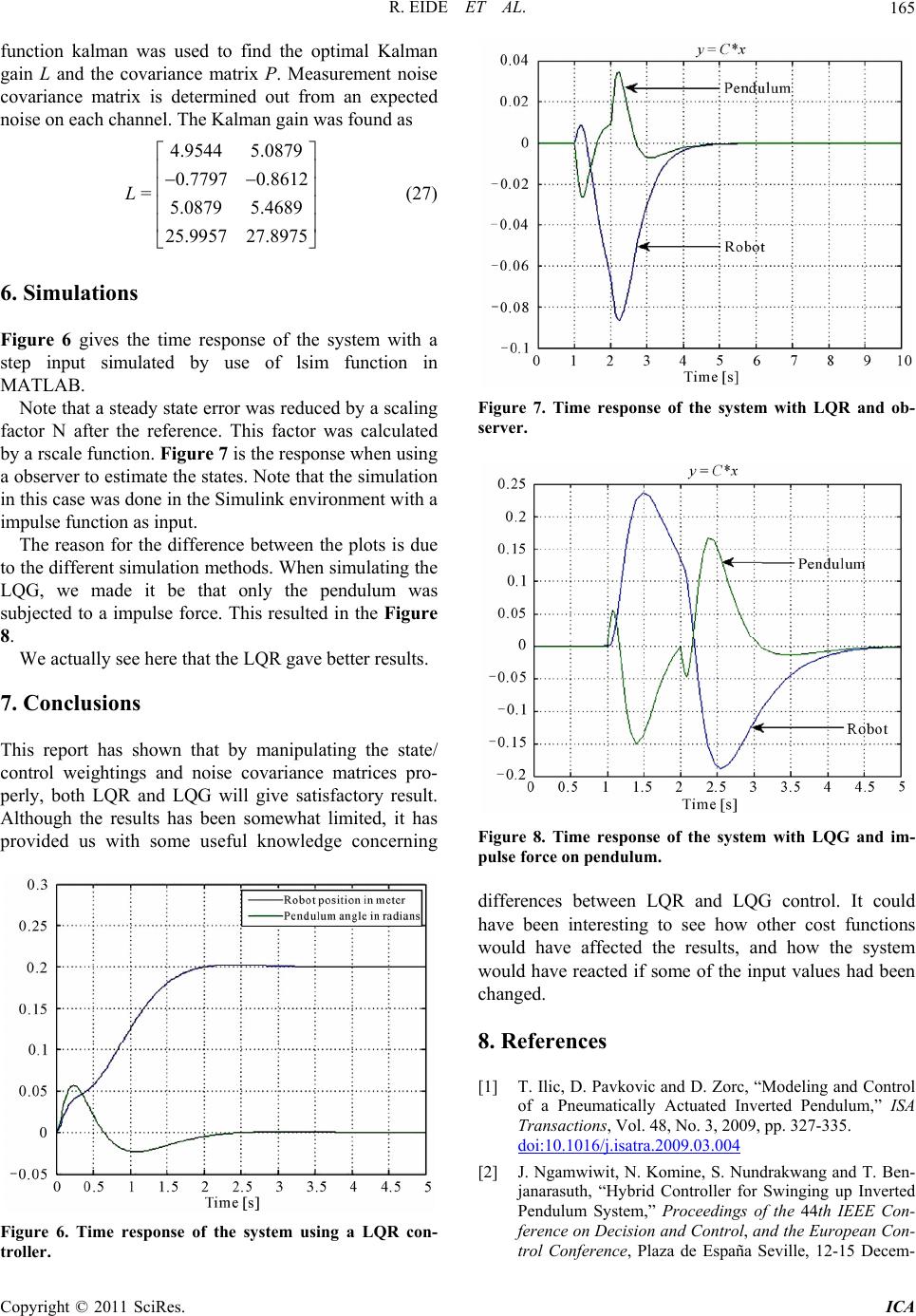
schemes beyond just stabilization. Thus, an observer is
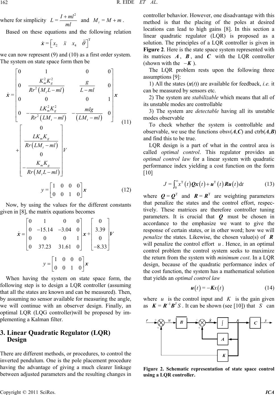
re e schematics of the
stem with the observer is shown in Figure 3 below.
from Figure 3, the observer state
eq
lied upon to supply accurate estimations of the states at
all robot-pendulum positions. Th
syAs can be seen
uations are g i v en by
ˆˆ ˆ
=
AxBuL yCx
(17)
ˆˆ
=yCx
(18)
where ˆ
is the estimate of the actual state
. Further-
more, Equations (17) and (18) can be re-written to
become
ˆˆ
=
ALCxBuLy
(19)
This, in turn, is the governing equations for a full
order observer, having two inputs u and y and one
output, ˆ
. Since we already know and servers
of this ki is simple in design a
estimation of all the states around t
From 3 we can se
difference between the mea
estimauts and correct the mde
Th
A, B
nd
o
u, ob
nd
Figure
ted outp
provides accurate
he linearized point.
e that the observer is im-
plemented by using a duplicate of the linearized system
dynamics and adding in a correction term that is simply a
gain on the error in the estimates. Thus, we will feed
back the sured and the
l continuously.
e proportional observer gain matrix,
, can be found
by pole placement method by use of e placecommand
in MATLAB. The poles were determined to be ten times
faster than the system poles. These were found to be
T
*=18.0542, 5.4482, 3.4398, 2.4187eig ABK,
which yields the gain matrix
34.4 0.2
91.0 1.1
=30.4 52.5
1103.6 726.4
th
L (20)
When combining the control-law design with the esti-
mator design we can get the compensator (see Section 6
for results).
4. Kalman Filter Desig
n
In the previous design of the state observer, the mea-
surements =
Cx
is not usually the case in
were assumed to be
practical li
inputs yielding the state equations to be on the general
stochastic state space form
noise free. This
fe. Other unknown
=
=
AxBu Gd
yCxHdn
(21)
where the matrices can be set to an identity matrix,
G
can be set toro, is stationary, zero mean zed
Copyright © 2011 SciRes. ICA