Intelligent Control and Automation, 2011, 2, 144-151
doi:10.4236/ica.2011.22017 Published Online May 2011 (http://www.SciRP.org/journal/ica)
A Measure Theoretical Approach for Path Planning
Problem of Nonlinear Control Systems
Amin Jajarmi1, Hamidreza Ramezanpour2, Mohammad Dehghan Nayyeri3, Ali Vahidian Kamyad3
1Department of Electrical Engineering, Ferdowsi University of Mashhad, Mashhad, Iran
2Department of Nuclear Engineering and Physics, AmirKabir University of Technology, Tehran, Iran
3Department of Applied Mathematics, Ferdowsi University of Mashhad, Mashhad, Iran
Received October 19, 2010; revised May 13, 2011; accepted May 15, 2011
Abstract
This paper presents a new approach to find an approximate solution for the nonlinear path planning problem.
In this approach, first by defining a new formulation in the calculus of variations, an optimal control problem,
equivalent to the original problem, is obtained. Then, a metamorphosis is performed in the space of problem
by defining an injection from the set of admissible trajectory-control pairs in this space into the space of
positive Radon measures. Using properties of Radon measures, the problem is changed to a measure-theo-
retical optimization problem. This problem is an infinite dimensional linear programming (LP), which is ap-
proximated by a finite dimensional LP. The solution of this LP is used to construct an approximate solution
for the original path planning problem. Finally, a numerical example is included to verify the effectiveness of
the proposed approach.
Keywords: Path Planning, Optimal Control, Measure Theory, Linear Programming
1. Introduction
In the control theory, the path planning problem finds an
admissible control for steering the control system from
an initial state to a desired final state in a certain finite
time interval. This problem has been developed initially
by the aerospace industries for trajectory modification of
aircrafts and space vehicles [1]. Moreover, it is one of the
most applicable control problems, especially in robot
industrial and etc [2-4]. However, the inherent nonlinear-
ity of practical systems presents a challenging path plan-
ning problem. For many systems, the conventional trial
and error method can work quite well to find system
schedules. But for more advanced ones, more accurate
methodologies are needed. For instance, in [5] the prob-
lem of optimal path planning has been considered as a
semi- infinite constrained optimization problem.
In the filed of path planning, many different solution
methods have been developed [6]. Most of the conven-
tional methods, such as road mapping [7] and potential
field [8], have some weaknesses in common. In the road
mapping method, which is probabilistic, the heuristic
nature of path generation leads to the difficulty in char-
acterizing the algorithm in terms of performance, com-
plexity, and reliability [9]. Potential field path planning
method has been appeared frequently in the literatures;
however, it has been plagued with inherent limitations
[10].
In [11] a chaotic genetic algorithm has been used to
find the shortest path for a mobile robot to move in a
static environment. Besides, in [12] a chaotic particle
swarm optimization (PSO) algorithm with mutation op-
erator has been employed in the path planning. But, since
the path planning is a complex NP-hard problem, general
particle swarm optimizer is slow in convergence and is
easy to be trapped in local optima, especially in complex
multi-apex search problem. In [13] a variational ap-
proach has been proposed for path planning in three di-
mensions by defining an energy integral over the path,
using gradient flow on the defined energy, and evolving
the entire path until a locally optimal steady state is
reached. A mixed integer linear programming (MILP)
method has also been proposed in [14,15] which yields
an optimization-based technique and performs quite well
in specific instances. This method combines linear pro-
gramming (LP) problem with the ability of constraining
some subset of the state variables to be integers.
In the past few years, the idea of finding solutions of

A. JAJARMI ET AL.145
some problems by converting them to a suitable optimal
control problem has received growing attentions. In
[16-18] you can see some applications of this idea for
solving a number of ordinary and partial differential
equations. The path planning problem can also be con-
verted to an optimal control problem by considering a
suitable objective function. Therefore, optimal control
concepts can be used which present a systematic ap-
proach to solve the problem. In [19], a new optimal con-
trol problem, equivalent to the path planning problem,
has been obtained by defining a new formulation in the
calculus of variations. Discretizing this new problem
yields a nonlinear programming (NLP) which may have
a large number of variables and a large number of con-
straints. To overcome this difficulty and reduce the
computational complexity, an iterative algorithm has also
been introduced in [19] in which a sequence of reduced
order NLP’s is solved instead of directly solving the
large NLP obtained through the discretization. However,
solving NLP problems is much more difficult than solving
LP ones.
In [20] a suitable tool is introduced to obtain approxi-
mate solutions for optimal control problems using the
concept of measure theory [21-23]. In this approach, to
find an acceptable solution, only a LP problem should be
solved. Therefore, the approach has the advantage that it
sets aside completely the nonlinearity of the problem.
Moreover, it does not depend on the convexity of objec-
tive function. Besides, it is practical for systems with too
complicated nonlinear terms.
In this paper, using the concept of measure theory, a
novel practical approach is proposed to approximate the
solution of nonlinear path planning problem. The pro-
posed approach in comparison with other numerical me-
thods works well; especially it is practical and accurate
enough for systems with too complicated nonlinear terms.
Moreover, as the obtained control function is piecewise
constant, it is suitable for switching systems. Besides,
error is completely controllable and accuracy can be im-
proved as fine as desired.
The paper is organized as follows. Section 2 defines
the problem of path planning, and Section 3 proposes a
new formulation for this problem. In Section 4, a meta-
morphosis is performed to convert the problem to an
infinite-dimensional LP in measure space. Then, by in-
troducing two stage approximations in Section 5, a fi-
nite-dimensional LP is obtained. In Section 6, an illustra-
tive example is presented to verify the effectiveness of
the proposed approach. Finally, conclusions are given in
the last section.
2. Definition
Consider the following general form of nonlinear path
planning problem:




 
 

,,
s.t.
,
,
,
aabb
ab
x
tgxtutt
xtAut U
x
txxtx
tJ tt





(1)
where


:n
x
JR is the state trajectory which is as-
sumed to be absolutely continuous on
J
and be con-
strained to stay in the compact set n
A
R,


:uJm R is the control function which is a bounded
measurable function on
J
and takes its values in the
compact set ,
m
UR


:
g
V is a continuous
function where V is a compact set and
n
R
A
UJ

, a
x
A

and b
x
A are the initial and
final states, respectively. In addition, it is assumed that
()
x
t satisfies the differential equation of system, almost
everywhere on
J
. Path planning problem is the problem
of guiding control system from the known initial state a
x
at 0a tt

to the given final state
b
x
at
f
b
Remark 1.1. Under the above-mentioned assumptions,
the nonlinear system in (1) without the final condition
tt.


bb
x
tx

has a unique solution

x
t

ut
for every bound-
ed measurable control function [24]. In this situa-
tion, under assumption that
g
x

 be continuous on

,
the solution of system obtained from a piecewise con-
tinuous control function


ut is piecewise function,
i.e.
1
C


x
t is continuous piecewise differentiable and has
piecewise continuous derivative [24].
3. New Formulation
In [25], there is a new formulation for the path planning
problem of linear time-varying systems. Here, that for-
mulation is extended for the nonlinear system in (1) by
defining a function
F
as follows:
    
21
:
(,,,) ,,
nm
FR R
F
xtxt ut txtgxt utt
 





 (2)
where

is a suitable continuous norm on and
n
R


0,R

. Now the following variational problem can
be defined:




 
 
min ,,,d
s.t.
,
, ,
J
aabb
F
xtxt ut tt
xtAut U
x
txxtxtJ



(3)
where
A
, , and U
J
are as before.

A. JAJARMI ET AL. 146


0

0
Problem (3) is equivalent to the original problem (1)
as the following theorem states:
Theorem 3.1. Problem (1) has a solution if and only if
problem (3) has an optimal solution with the corre-
sponding zero optimal objective value.
Proof. The “only if” part is obvious. For the “if” part
let be the optimal solution of problem (3)
with corresponding zero optimal objective value, that is


**
,xu
  

***
,,,d
J
Fx tx t u t tt
. Since the integrand is
nonnegative real-valued function, we have
 

***
,,,Fxtxtutt  almost everywhere on
J
,
and so almost everywhere
 

**
xt gxtu


0
*
,,tt
on
J
, and

a
*
a
x
tx and

b
*
b
x
tx. As
  
td
a
at
x
txt xs


s

for t and J


x
t

 is
Lebesgue integrable,

x
t


*
,xu
 will be absolutely continu-
ous and therefore is a solution of problem

*


(1). Thus, the proof is complete.
Introducing slack variable




vt xt
 , problem (3)
can be expressed as an optimal control problem as fol-
lows:


 
 
  
 
min ,,,d
s.t.
, ,
, ,
J
aabb
F
xt vt ut tt
xt vt
x
tAutUvtV
x
txxtxtJ




 (4)
where
A
, , , and U V
J
are as before. It is easy to
show that problems (3) and (4) are equivalent.
Consider


vt

as a new control vector and define
 

ˆut ut vt



 . Therefore, problem (4) can be rewritten
as:


 
  
 
 
ˆˆ
min ,,d
s.t.
ˆ 0I
ˆ
ˆ ,
, ,
J
nm nn
aabb
Fxt ut tt
xt, ut
xtAut U
x
txxtxtJ







(5)
where
  

 
ˆˆ
,, ,,,
F
xt ut tFxt vt ut t
nm
V R


and
.
ˆ
UU
Definition 3. 1. The trajectory-control pair
in problem (5) is called admissible if the
following conditions hold:
  
ˆ , wxu 

1)


x
 is absolutely continuous on
J
and satisfies

,
x
tAtJ.
2)


ˆ
u

is bounded Lebesgue measurable on
J
and
takes its values in .
ˆ
U
3) Boundary conditions

aa
x
tx and


bb
x
tx

are satisfied.
4) The state equation

 


ˆ
0I
nm nn
x
t,u


t is satis-
fied.
Let be the set of all admissible pairs. Then, prob-
lem (5) (and equivalently (1), (3) and (4)) has a solution
when is non-empty.
W
W
Some characteristics of the admissible pairs are as fol-
lows. Let






ˆ
, wxu


R
be an admissible pair, and
be an open ball in containing B1n
A
J

. Let
()CB

be the space of all real-valued functions that are
uniformly continuous on together with their first
derivatives. Let
B


CB 

 and define function


as
follows:





 

 

 
   
ˆ
,, ,,
ˆ ,, ,
xt
x
tuttxttvtxtt
xt ut tCB







(6)
where ˆ
A
UJ

. Also,


is in the space


C

,
of real valued continuous functions defined on the com-
pact set

. Since




wx ˆ ,u

 is admissible pair, for
all


CB 

 we have:






    




ˆ ,,d
,,d
,d ,,
J
xt
J
bb aa
J
xt ut tt
xt tvtxt tt
xtttx tx t










(7)
Note that it is necessary to introduce the set and the
space
B


CB
 since
A
may have an empty interior in
. Now, consider
n
R


j
x
t and as the components
of

j
vt


x
t and


vt , respectively. Let be the
space of infinitely differentiable real-valued functions
with compact support in


DJ

,
ab

J
tt
. Define:






 



ˆ ,,
1,2,, ,
jjj
x
tuttxt tvt t
jnDJ









(8)
Then, if






ˆ
,
wxu

 is an admissible pair, for
1, 2,,jn

 and


DJ   we have:
 

  


    

 

  
   


ˆ
,,d d
d
dd
d
d0
jjj
JJ
jjj
j
J
jjj
J
jJjj
J
xt ut ttx ttv ttt
x
ttxttxttvtt
xt t xt tvt tt
t
xttxtvtt t










 








t

(9)

A. JAJARMI ET AL.147
since the function

has compact support in
J
, i.e.
, and the trajectory and control func-
tions in an admissible pair satisfy the state equation in (5).
 
0
ab
tt  
Now, consider a special choice of function

in
which depends on the time variable only, i.e.

CB


,
 
x
tt t
 
ˆ
,,
ut t 


xt

 . In the light of (6) we have
 
1
t C  
 where is a sub-

1
C
space of comprised of those continuous functions
which depend only on the time variable. In addition, (7)
implies that:

C
  

  

1
ˆ
,,dd ba
JJ
x
tutt ttttt
C










(10)
The set of Equalities (7), (9) and (10) are the properties
of admissible pairs in the new but classical formulation of
the path planning problem. In the next section, by suitable
generalization, a transformation into another, non-clas-
sical problem is introduced which has better properties in
some aspects.
4. Metamorphosis
For each admissible pair
  
ˆ
,wxu

 consider the
following well-defined mapping:
 


ˆ
:,
w
J
,d
H
CHxtutttR

 
 (11)
This mapping is a bounded linear functional on


C

which is also positive, i.e. w assigns nonnegative val-
ues to the nonnegative continuous functions

H
on

.
Proposition 4.1. Let
g
x

 be continuous on

and

ut be piecewise continuous on
J
. The transformation
from W, the set of admissible pairs
, into the space of bounded linear func-
tional on is an injection.
w
 

w
wx

ˆ
,u

C


Proof. It must be shown that if
, then .
Indeed, if 12
, then by relation (5), 12
   
11 12 22
ˆˆ
,,wxuw xu  
ww12
ww

x
x. Since
1
x
and 2
x
are continuous, there is a subinterval 1
J
J

such that
 
12 1
,
x
txt tJ. Now, a continuous
function
H
can be constructed such that it is equal zero
for all outside 1 t
J
and positive on the appropriate
portion of the graph of

1
x
 and zero on that of


2
x

.
Then,

12
ww
H
H

, and the proof is complete.
Let be a linear positive continuous functional on
. By Riesz representation Theorem, there exists a
unique positive Radon measure

C


on such that:


d, HH HHC 

 
 (12)
It is said that

is a representing measure for

. Let


M

be the space of all positive Radon measure on

. Then, solving problem (5) is equivalent to seek a
measure in


M

, denoted by *

, which minimizes
the functional:
ˆ)() (
M
F  R 


  (13)
over the set w Q of the measures

, corresponding to
the admissible pairs
 


ˆ
, wxu

, which satisfy:




0,
,
j
f
fa







1
,
1, 2,,,
CB
jnD
fC
 

  
 


J   (14)
Existence of the optimal measure *

in the set is
equivalent to the controllability of problem (1). If is
compact, then existing of the optimal measure
w
Q
w
Q
*

is
guaranteed, as the map

ˆ, w
F
Q    , mapping
w into the real line, is continuous, where w is con-
sidered to have relative topology induced by the topol-
ogy of
Q Q



M

. But in general w may not be com-
pact. However, if we extend w to the set includ-
ing all measures in
Q
Q Q


M which satisfy (14) (not
necessarily those measures corresponding to the admis-
sible pairs), then the optimal measure *

in exists
which is shown by the following theorem:
Q
Theorem 4.1. Let be the set of all posi-
tive Radon measure on

QM





satisfying (14). There exists an
optimal measure *

in the set for which Q




ˆˆ
F
F 
, for all Q


.
Proof. It is similar to the proof of Theorem II.1 in [20]
and we neglect it.
Notice that in this case, which the set w is extended
to the set ,
Q
Q*

is not necessarily a measure corre-
sponding to an admissible pair .
w
Remark 4.1. Minimization of functional (13) subject to
(14) is an infinite-dimensional LP. But it is possible to
approximate the solution of this problem by the solution
of a finite-dimensional LP of sufficiently large dimension
which will be done in the next section.
5. Approximation
For the first step of approximation, we consider the
measures in


M

satisfying a finite number of con-
straints in (14). To do this, let and

1
:1,2,,kM  
k


2
,2,,:1hM
h
  be subsets of some total sets in


CB
 and


DJ
, respectively (A subset of


C
B
or


DJ
 is total if the linear combinations of its ele-
ments be dense in that space).
Theorem 5.1. Consider LP consisting of minimizing
the function


ˆ
F
  over the set


12
,QM M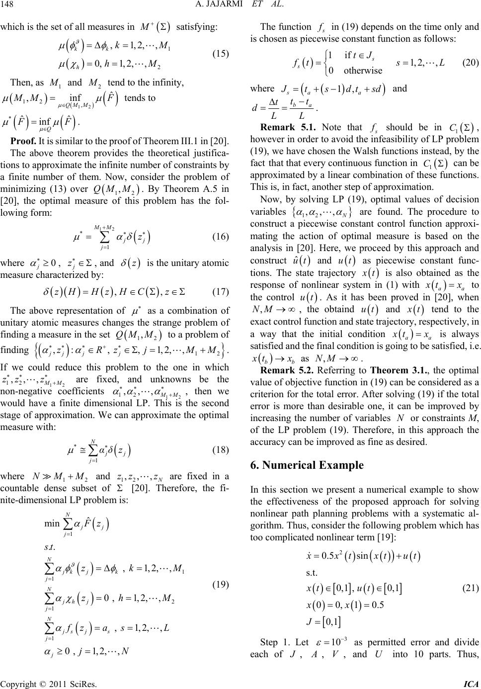

A. JAJARMI ET AL. 148
which is the set of all measures in satisfying:

M
1
2
2,,
,
kM
hM




, 1,
0, 1,2,
kk
h

 


 (15)
Then, as 1
M
and 2
M
tend to the infinity,



12
12 ,
ˆ
,inf
QM M
M
MF



 tends to
 
*ˆˆ
inf
Q
F
F



.
Proof. It is similar to the proof of Theorem III.1 in [20].
The above theorem provides the theoretical justifica-
tions to approximate the infinite number of constraints by
a finite number of them. Now, consider the problem of
minimizing (13) over 12 . By Theorem A.5 in
[20], the optimal measure of this problem has the fol-
lowing form:

,QM M


12
*
1
MM
j
j
z 
j





 (16)
where , j, and 0
j

z


z 
is the unitary atomic
measure characterized by:

zH HzH  

, ,Cz (17)
The above representation of

 as a combination of
unitary atomic measures changes the strange problem of
finding a measure in the set


12
,M
, , 1,2,j
QM

to a problem of
finding .

12
, :,
jj jj
zRz MM 
  
 


If we could reduce this problem to the one in which
12
12
,, ,
M
M
zz z
 

 are fixed, and unknowns be the
non-negative coefficients 12
12
,,,
M
M, then we
would have a finite dimensional LP. This is the second
stage of approximation. We can approximate the optimal
measure with:







*
1
N
j
j
j
αδ z 


 (18)
where 12 and NMM12 ,, ,
N
zz

z
2
, 1
,2, ,
,2,,
1,2,,L



are fixed in a
countable dense subset of [20]. Therefore, the fi-
nite-dimensional LP problem is:




1
1
1
1
1
ˆ
min
..
0 , 1
,
0 , 1,2,,
N
jj
j
N
jk jk
j
N
jh j
j
N
js js
j
j
Fz
st
zk
zh M
fzas
jN


 
















The function
s
f
in (19) depends on the time only and
is chosen as piecewise constant function as follows:

1 if 1,2,,
0 otherwise
s
s
tJ
f
ts





L (20)
where




1,
sa a
J
tsdtsd and
ba
tt
t
dLL


 .
Remark 5.1. Note that
s
f
should be in


1
C

,
however in order to avoid the infeasibility of LP problem
(19), we have chosen the Walsh functions instead, by the
fact that that every continuous function in


1
C

can be
approximated by a linear combination of these functions.
This is, in fact, another step of approximation.
Now, by solving LP (19), optimal values of decision
variables


12
,,,
N

  are found. The procedure to
construct a piecewise constant control function approxi-
mating the action of optimal measure is based on the
analysis in [20]. Here, we proceed by this approach and
construct


ˆ
ut and


ut as piecewise constant func-
tions. The state trajectory

x
t is also obtained as the
response of nonlinear system in (1) with a

a
x
tx

to
the control


ut . As it has been proved in [20], when
, the obtaind and ,NM

ut

x
t

a
tend to the
exact control function and state trajectory, respectively, in
a way that the initial condition a
x
tx is always
satisfied and the final condition is going to be satisfied, i.e.


bb
x
tx,NM as .
Remark 5.2. Referring to Theorem 3.1., the optimal
value of objective function in (19) can be considered as a
criterion for the total error. After solving (19) if the total
error is more than desirable one, it can be improved by
increasing the number of variables or constraints M,
of the LP problem (19). Therefore, in this approach the
accuracy can be improved as fine as desired.
N
6. Numerical Example
In this section we present a numerical example to show
the effectiveness of the proposed approach for solving
nonlinear path planning problems with a systematic al-
gorithm. Thus, consider the following problem which has
too complicated nonlinear term [19]:

  
   
 

2
0.5 sin
s.t.
0,1, 0,1
00, 10.5
0, 1
x
xtxtut
xt ut
xx
J





(21)
M
(19)
Step 1. Let 3 10 

 as permitted error and divide
each of
J
,
A
, , and U into 10 parts. Thus, V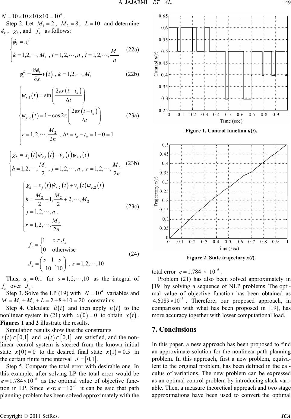

A. JAJARMI ET AL.149
4
10 10 10 1010N 
2MM
k
.
Step 2. Let 1, 2, and determine 810L

, h

, and
s
f
as follows:
1
1
1,2,, , 1,
j
ki
x
2,, , 1,2,,
M
kMi





nj n
 
(22a)

1
, 1,2,,
k
kvt kM
x





 (22b)




,1
,2
2
2π
sin
2π
1cos2π
1,2,, , 101
2
a
r
a
r
ba
rt t
tt
rt t
tt
M
rttt
n











 


 





(23a)
 
,1 ,1
22
1,2,,,1,2,, , 1,2,,
22
hj rjr
xt tvt t
M
M
hjnr
n
   






(23b)
  
,2 ,2
22
2
2
1,2, ,
22
1,2,, ,
1, 2,,2
hj rjr
x
ttvt
MM
hM
jn
M
rn
  












t
(23c)
1
0 otherwise
1, , 1,2,,1
10 10
s
s
s
zJ
f
ss
Js








 0
(24)
Thus, for as the integral of 0.1
s
a1,2,,10s
s
f
over
s
J
.
Step 3. Solve the LP (19) with variables and
constraints.
4
10
20
N
12
Step 4. Calculate and then apply to the
nonlinear system in (21) with to obtain
2810MM ML

ˆ ut

ut

00x


x
t.
Figures 1 and 2 illustrate the results.
Simulation results show that the constraints
 

0,1xt  and
 

0, 1ut are satisfied, and the non-
linear control system is steered from the known initial
state to the desired final state in
the certain finite time interval

0x0

10.5x


0,1J.
Step 5. Compare the total error with desirable one. In
this example, after solving LP the total error would be
as the optimal value of objective func-
tion in LP. Since
6
1.784 10e 
3
10e 

 it can be said that path
planning problem has been solved approximately with the
Figure 1. Control function u(t).
Figure 2. State trajectory x(t).
total error 6 1.784 10e

.
Problem (21) has also been solved approximately in
[19] by solving a sequence of NLP problems. The opti-
mal value of objective function has been obtained as
5
4.6089 10

. Therefore, our proposed approach, in
comparison with what has been proposed in [19], has
more accuracy together with lower computational load.
7. Conclusions
In this paper, a new approach has been proposed to find
an approximate solution for the nonlinear path planning
problem. In this approach, first a new problem, equiva-
lent to the original problem, has been defined in the cal-
culus of variations. The new problem can be expressed
as an optimal control problem by introducing slack vari-
able. Then, a measure theoretical approach and two stage
approximations have been used to convert the optimal

A. JAJARMI ET AL. 150
control problem to a finite dimensional LP. The solution
of this LP is used to construct an approximate solution
for the original path planning problem. The proposed
approach in comparison with other numerical methods
works well; especially it is practical and accurate enough
for systems with too complicated nonlinear terms.
Moreover, error is completely controllable and accuracy
can be improved as fine as desired. In addition, as the
obtained control function is piecewise constant, it is
suitable for switching systems. Effectiveness of the pro-
posed approach has been verified using a numerical ex-
ample.
8. Acknowledgements
The authors gratefully acknowledge the helpful com-
ments and suggestions of the reviewers, which have im-
proved the manuscript.
9. References
[1] J. M. Athans and P. L. Falb, “Optimal Control: An Intro-
duction to the Theory and Its Applications,” McGraw-
Hill, New York, 1996.
[2] A. T. Hasan, A. M. S. Hamouda, N. Ismail and H. M. A.
A. Al-Assadi, “A New Adaptive Learning Algorithm for
Robot Manipulator Control,” Proceedings of the Institu-
tion of Mechanical Engineers Part I-Journal of Systems
and Control Engineering, Vol. 221, No. 4, 2007, pp.
663-672. doi:10.1243/09596518JSCE321
[3] A. S. Rana and A. M. S. Zalzala, “Collision-Free Motion
Planning of Multi-Arm Robots Using Evolutionary Algo-
rithms,” Proceedings of the Institution of Mechanical En-
gineers Part I-Journal of Systems and Control Engineer-
ing, Vol. 211, No. 5, 1997, pp. 373-384.
doi:10.1243/0959651971539902
[4] C. L. Chen and C. J. Lin, “Motion Planning of Redundant
Robot Manipulators Using Constrained Optimization: A
Parallel Approach,” Proceedings of the Institution of
Mechanical Engineers Part I-Journal of Systems and
Control Engineering, Vol. 212, No. 4, 1998, pp. 281-292.
doi:10.1243/0959651981539460
[5] Y. Wang, D. M. Lane and G. J. Falconer, “Two Novel
Approaches for Unmanned under Water Vehicle Path
Planning: Constrained Optimization and Semi-Infinite
Constrained Optimization,” Robotica, Vol. 18, No. 2,
2000, pp. 123-142.
doi:10.1017/S0263574799002015
[6] J. C. Latombe, “Robot Motion Planning,” Kluwer Aca-
demic Publishers, Boston, 1991.
[7] L. Kavarki, P. Svestka, J. Latombe and M. Overmars,
“Probabilistic Road Maps for Path Planning in High Di-
mensional Configuration Space,” IEEE Transactions on
Robotics and Automation, Vol. 12, No. 4, 1996, pp.
566-580. doi:10.1109/70.508439
[8] G. C. Luh and W. W. Liu, “Motion Planning for Mobile
Robots in Dynamic Environments Using a Potential Field
Immune Network,” Proceedings of the Institution of Me-
chanical Engineers Part I-Journal of Systems and Con-
trol Engineering, Vol. 221, No. 7, 2007, pp. 1033-1045.
doi:10.1243/09596518JSCE400
[9] L. Kavarki, M. Kolountzakis and J. Latombe, “Analysis
of Probabilistic Road Maps for Path Planning,” IEEE
Transactions on Robotics and Automation, Vol. 14, No. 1,
1998, pp. 166- 171. doi:10.1109/70.660866
[10] Y. Koren and J. Borenstein, “Potential Field Methods and
Their Inherent Limitations for Mobile Robot Navigation,”
Proceedings of the IEEE Conference on Robotics and
Automation, Sacramento, 1991.
doi:10.1109/ROBOT.1991.131810
[11] P. C. Zhou, B. R. Hong and J. H. Yang, “Chaos Genetic
Algorithm Based Path Planning Method for Mobile Ro-
bot,” Journal of Harbin Institute of Technology, Vol. 36,
No. 7, 2004, pp. 880-883.
[12] Y. O. Qin, D. B. Sun, N. Li and Y. G. Cen, “Path Plan-
ning for Mobile Robot Using the Particle Swarm Opti-
mization with Mutation Operator,” Proceedings of the
3rd International Conference on Machine Learning and
Cybernetics, Shanghai, 2004.
[13] T. Cecil and D. E. Marthaler, “A Variational Approach to
Path Planning in Three Dimensions Using Level Set
Methods,” Journal of Computational Physics, Vol. 211,
No. 1, 2006, pp. 179-197.
doi:10.1016/j.jcp.2005.05.015
[14] M. G. Earl and R. Danderia, “Modelling and Control of a
Multi-Agent System Using Mixed Integer Linear Pro-
gramming,” Proceedings of the 41st IEEE Conference on
Decision and Control, Las Vegas, 10-13 December 2002.
doi:10.1109/CDC.2002.1184476
[15] A. Richards and J. How, “Aircraft Trajectory Planning
with Collision Avoidance Using Mixed Integer Pro-
gramming,” Proceedings of the IEEE American Control
Conference, Anchorage, Alaska, 2002.
[16] M. Gachpazan and A. V. Kamyad, “Solving of Second
Order Nonlinear PDE Problems by Using Artificial Con-
trols with Controlled Error,” Korean Journal of Compu-
tational & Applied Mathematics, Vol. 15, No. 1-2, 2004,
pp. 173-184.
[17] S. A. Alavi, A. V. Kamyad and M. Gachpazan, “Solving
of Nonlinear Ordinary Differential Equations as a Control
Problem by Using Measure Theory,” Scientia Iranica,
Vol. 7, No. 1, 2000, pp. 1-7.
[18] M. Gachpazan, A. Kerayechian and A. V. Kamyad, “A
New Method for Solving Nonlinear Second Order Dif-
ferential Equations,” Korean Journal of Computational &
Applied Mathematics, Vol. 7, No. 2, 2000, pp. 333-345.
[19] A. Jajarmi, M. Gachpazan and A. V. Kamyad, “Open-
loop Control of Nonlinear Systems via a Sequence of
Nonlinear Programming Problems,” Proceedings of the
17th Iranian Conference of Electrical Engineering, Te-
hran, 13-15 August 2009.
[20] J. E. Rubio, “Control and Optimization, the Linear

A. JAJARMI ET AL. 151
Treatment of Non-linear Problems,” Manchester Univer-
sity Press, Manchester, 1986.
[21] A. V. Kamyad, J. E. Rubio and D. A. Wilson, “An Opti-
mal Control Problem for the Multidimensional Diffusion
Equation with a Generalized Control Variable,” Journal
of Optimization Theory and Applications, Vol. 75, No. 1,
1992, pp. 101-132. doi:10.1007/BF00939908
[22] A. V. Kamyad and A. H. Borzabadi, “Strong Controlla-
bility and Optimal Control of the Heat Equation with a
Thermal Source,” Korean Journal of Computational &
Applied Mathematics, Vol. 7, No. 3, 2002, pp. 555-568.
[23] A. H. Borzabadi, A. V. Kamyad and M. H. Farahi, “Op-
timal Control of the Heat Equation in an Inhomogeneous
Body,” Applied Mathematics and Computation, Vol. 15,
No. 1-2, 2004, pp. 127-146.
[24] D. Hinrichsen and A. J. Pritchard, “Mathematical System
Theory I: Modeling, State Space Analysis, Stability and
Robustness,” Springer, Berlin, 2005.
[25] A. V. Kamyad and H. H. Mehneh, “A Linear Program-
ming Approach to the Controllability of Time-Varying
Systems,” International Journal of Engineering Science,
Vol. 14, No. 8, 2003, pp. 143-151.