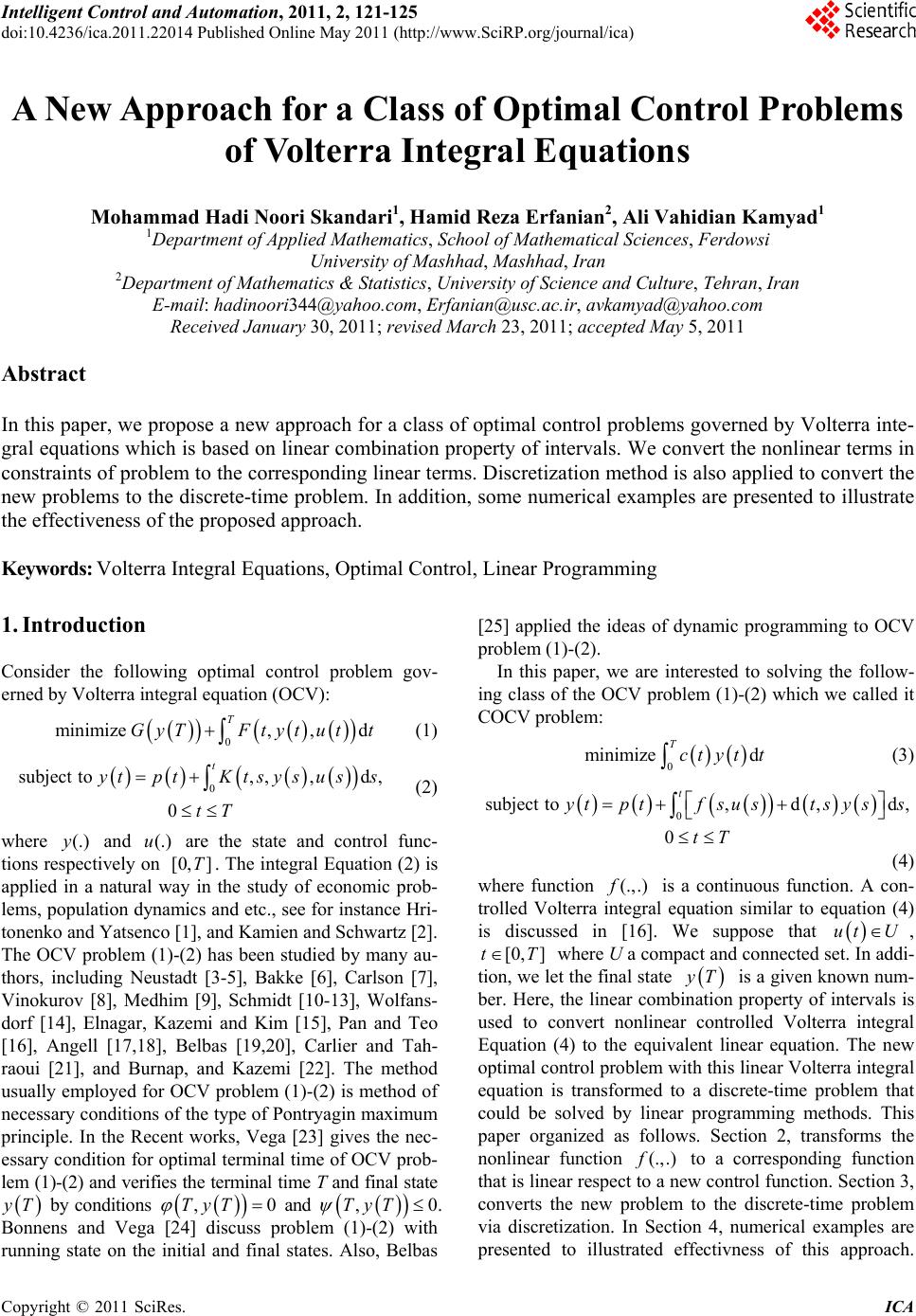
 Intelligent Control and Automation, 2011, 2, 121-125 doi:10.4236/ica.2011.22014 Published Online May 2011 (http://www.SciRP.org/journal/ica) Copyright © 2011 SciRes. ICA A New Approach for a Class of Optimal Control Problems of Volterra Integral Equations Mohammad Hadi Noori Skandari1, Hamid Reza Erfanian2, Ali Vahidian Kamyad1 1Department of Applied Mathematics, School of Mathematical Sciences, Ferdowsi University of Mashhad, Mashhad, Iran 2Department of Mathematics & Statistics, University of Science and Culture, Tehran, Iran E-mail: hadinoori344@yahoo.com, Erfanian@usc.ac.ir, avkamyad@yahoo.com Received January 30, 2011; revised March 23, 2011; accep t e d M ay 5, 2011 Abstract In this paper, we propose a new approach for a class of optimal control problems governed by Volterra inte- gral equations which is based on linear combination property of intervals. We convert the nonlinear terms in constraints of problem to the corresponding linear terms. Discretization method is also applied to convert the new problems to the discrete-time problem. In addition, some numerical examples are presented to illustrate the effectiveness of the proposed approach. Keywords: Volterra Integral Equations, Optimal Control, Linear Programming 1. Introduction Consider the following optimal control problem gov- erned by Volterra integral equation (OCV): 0 minimize, ,d T GyTFtyt utt (1) 0 subject to,,,d, 0 t tpt Ktsysuss tT (2) where and are the state and control func- tions respectively on . The integral Equation (2) is applied in a natural way in the study of economic prob- lems, population dynamics and etc., see for instance Hri- tonenko and Yatsenco [1], and Kamien and Schwartz [2]. The OCV problem (1)-(2) has been studied by many au- thors, including Neustadt [3-5], Bakke [6], Carlson [7], Vinokurov [8], Medhim [9], Schmidt [10-13], Wolfans- dorf [14], Elnagar, Kazemi and Kim [15], Pan and Teo [16], Angell [17,18], Belbas [19,20], Carlier and Tah- raoui [21], and Burnap, and Kazemi [22]. The method usually employed for OCV problem (1)-(2) is method of necessary conditions of the type of Pontryagin maximum principle. In the Recent works, Vega [23] gives the nec- essary condition for optimal terminal time of OCV prob- lem (1)-(2) and verifies the terminal time T and final state (.)y(.)u [0, ]T T by conditions ,0T Ty and ,TyT 0 . Bonnens and Vega [24] discuss problem (1)-(2) with running state on the initial and final states. Also, Belbas [25] applied the ideas of dynamic programming to OCV problem (1)-(2). In this paper, we are interested to solving the follow- ing class of the OCV problem (1)-(2) which we called it COCV problem: 0 minimize d Tctyt t (3) 0 subject to,d,d, 0 t tptfsus tsyss tT (4) where function is a continuous function. A con- trolled Volterra integral equation similar to equation (4) is discussed in [16]. We suppose that (.,.)f ut U , [0, ]tT where U a compact and connected set. In addi- tion, we let the final state T is a given known num- ber. Here, the linear combination property of intervals is used to convert nonlinear controlled Volterra integral Equation (4) to the equivalent linear equation. The new optimal control problem with this linear Volterra integral equation is transformed to a discrete-time problem that could be solved by linear programming methods. This paper organized as follows. Section 2, transforms the nonlinear function to a corresponding function that is linear respect to a new control function. Section 3, converts the new problem to the discrete-time problem via discretization. In Section 4, numerical examples are presented to illustrated effectivness of this approach. (.f,.) 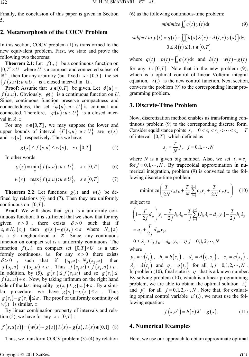 M. H. N. SKANDARI ET AL. 122 Finally, the conclusion of this paper is given in Section 5. 2. Metamorphosis of the COCV Problem In this section, COCV problem (1) is transformed to the new equivalent problem. First, we state and prove the following two theorems: Theorem 2.1: Let be a continuous function on where U is a compact and connected subset of , then for any arbitrary (but fixed) (.,.)f [0, ]TU m [0, ] T the set ,: suu U is a closed interval in . Proof: Assume that [0, ] T be given. Let u , su . Obviously, (.) is a continuous function on U. Since, continuous function preserve compactness and connectedness, the set is compact and connected. Therefore, is a closed inter- val in.□ :uu :uu U U For any [0, ] T, we may suppose the lower and upper bounds of interval ,: suu U are s and respectively. Thus we have: ws ,,0, sfsuwss T (5) In other words min, :,0, u sfsuuUsT (6) max, :,0, u wsf suuUsT (7) Theorem 2.2: Let functions (.) and be de- fined by relations (6) and (7). Then they are uniformly continuous on . (.)w [0,]T Proof: We will show that (.) is a uniformly con- tinuous function. It is sufficient that we show that for any given 0 , there exists 0 such that if 12 Ns then 12 gsgs where Nz is a (.,.f neighborhood of . Since, any continuous function on compact set is a uniformly continuous. The function on compact set is a uni- formly continuous, i.e. for any z )[0, ]TU 0 there exists 0 , such that if 12 ,, uNs u then 12 ,u f,sufs . Thus fsu 12 ,,suf . In addition, by (5), 11 , sfsu and so 1 gs 2,fsu . Now, by taking infimum on the right hand side of the last inequality gs 1 gs 2 gs 21 . By a simi- lar procedure, we havegs . Thus 12 gs gs . The proof of uniformly continuity of is similar. □ (.)w By linear combination property of intervals and rela- tion (5), we have for any [0, ] T: ,fsuswsgss gss ,[0,1] , (8) Thus, we transform COCV problem (3)-(4) by relation (6) as the following continuous-time problem: 0d T minimizectytt (9) 0,d 01,0, t ubject toytqthssdtsyss ttT where and 0d t qtptgs s htwtgt for any [0, ].tT Note that in the new problem (9), which is a optimal control of linear Volterra integral equation, (.) is the new control function. Next section, converts the problem (9) to the corresponding linear pro- gramming problem. 3. Discrete-Time Problem Now, discretization method enables us transforming con- tinuous problem (9) to the corresponding discrete form. Consider equidistance points 012 0N sssT of interval which defined as [0, ]T jT j N , 0,1,,jN where N is a given big number. Also, we set j ts for 0,1,,jN . By trapezoidal approximation in nu- merical integration, problem (9) is converted to the fol- lowing discrete-time problem: 1 00 1 minimize 22 N jj NN j TT T cycyc y NNN (10) 1 00 0 1 00 00 subject to 122 2 , 2 01,,0,1, 2,, j jji jiijj i jj jN TTTT dyhh dyh jjj j T qdy j yqy jN where j yyt, j hhs, , , ijij ddts j ccs, j t and j qqt for all . In problem (10), final state is ,0,1,2,,ij N that is a known number. By solving problem (10), which is a linear programming problem, we are able to obtain the optimal solution and y for all 0,1,2,,jN . Note that, for evaluat- ing optimal control variable , we must use the fol- lowing equation: (.u) ,. suhsgs (11) 4. Numerical Examples Here, we use our approach to obtain approximate optimal Copyright © 2011 SciRes. ICA 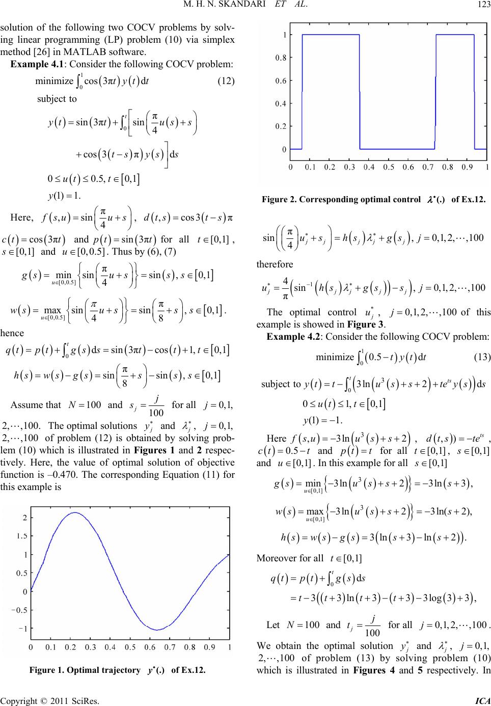 M. H. N. SKANDARI ET AL.123 solution of the following two COCV problems by solv- ing linear programming (LP) problem (10) via simplex method [26] in MATLAB software. Example 4.1: Consider the following COCV problem: 1 0 minimizecos 3πdtyt t (12) 0 subject to π sin 3πsin 4 cos3πd 00.5,0,1 (1) 1. t yttus s tsys s ut t y Here, π ,sin 4 suu s , ,cos3 πdtst s cos 3πct t andfor all sin 3πptt[0,1]t , and u. Thus by (6), (7) [0,1]s[0,0.5] [0,0.5] π min sinsin,0,1 4 u gsu sss [0,0.5] π max sinsin,0,1 48 u wsu sss . hence 0dsin3πcos1,0,1 t qtptgs sttt π sinsin ,0,1 8 hswsgsss s Assume that and 100N100 jj s for all 0,1,j 2, ,100. The optimal solutions y and , 0,1,j of problem (12) is obtained by solving prob- lem (10) which is illustrated in Figures 1 and 2 respec- tively. Here, the value of optimal solution of objective function is –0.470. The corresponding Equation (11) for this example is 2, ,100 Figure 1. Optimal trajectory of Ex.12. (.)y Figure 2. Corresponding optimal control of Ex.12. (.) π sin,0,1, 2,,100 4jjjj j ushsgs j therefore 1 4sin,0,1, 2,,100 π jjjjj uhsgssj The optimal control * u, of this example is showed in Figure 3. 0,1, 2,,100j Example 4.2: Consider the following COCV problem: 1 0 minimize 0.5dtyt t (13) 0 3 subject to3ln2d 01,0,1 (1) 1. tts yttu ssteyss ut t y Here ,3lnfsuu ss 32 , ,)dtste ts , ct 0.5 t and pt t for all , [0,1][0,1]st and [0,1]u . In this example for all [0,1]s [0,1] 3 min3ln23ln3 , u gsu sss [0,1] 3 max 3ln23ln(2), u wsu sss 3ln3ln2 .hsws gsss Moreover for all [0,1]t 0d 33ln3 33log33 t qtptgs s ttt t , Let 100N and 100 jj t for all . 0,1, 2,,100j We obtain the optimal solution y and , 0,1,j of problem (13) by solving problem (10) which is illustrated in Figures 4 and 5 respectively. In 2, ,100 Copyright © 2011 SciRes. ICA 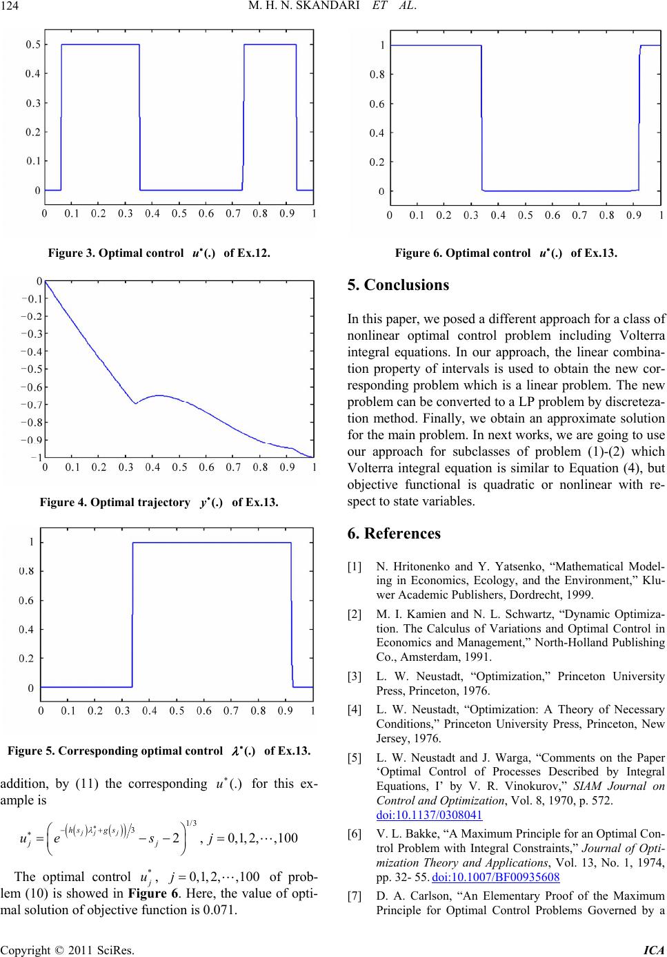 M. H. N. SKANDARI ET AL. 124 Figure 3. Optimal control of Ex.12. (.)u Figure 4. Optimal trajectory of Ex.13. (.)y Figure 5. Corresponding optimal control of Ex.13. (.) addition, by (11) the corresponding for this ex- ample is (.)u 1/3 32,0,1,2,,100 jj j hs gs jj ues j The optimal control * u, of prob- lem (10) is showed in Figure 6. Here, the value of opti- mal solution of objective function is 0.071. 0,1, 2,,100j Figure 6. Optimal control of Ex.13. (.)u 5. Conclusions In this paper, we posed a different approach for a class of nonlinear optimal control problem including Volterra integral equations. In our approach, the linear combina- tion property of intervals is used to obtain the new cor- responding problem which is a linear problem. The new problem can be converted to a LP problem by discreteza- tion method. Finally, we obtain an approximate solution for the main problem. In next works, we are going to use our approach for subclasses of problem (1)-(2) which Volterra integral equation is similar to Equation (4), but objective functional is quadratic or nonlinear with re- spect to state variables. 6. References [1] N. Hritonenko and Y. Yatsenko, “Mathematical Model- ing in Economics, Ecology, and the Environment,” Klu- wer Academic Publishers, Dordrecht, 1999. [2] M. I. Kamien and N. L. Schwartz, “Dynamic Optimiza- tion. The Calculus of Variations and Optimal Control in Economics and Management,” North-Holland Publishing Co., Amsterdam, 1991. [3] L. W. Neustadt, “Optimization,” Princeton University Press, Princeton, 1976. [4] L. W. Neustadt, “Optimization: A Theory of Necessary Conditions,” Princeton University Press, Princeton, New Jersey, 1976. [5] L. W. Neustadt and J. Warga, “Comments on the Paper ‘Optimal Control of Processes Described by Integral Equations, I’ by V. R. Vinokurov,” SIAM Journal on Control and Optimization, Vol. 8, 1970, p. 572. doi:10.1137/0308041 [6] V. L. Bakke, “A Maximum Principle for an Optimal Con- trol Problem with Integral Constraints,” Journal of Opti- mization Theory and Applications, Vol. 13, No. 1, 1974, pp. 32- 55. doi:10.1007/BF00935608 [7] D. A. Carlson, “An Elementary Proof of the Maximum Principle for Optimal Control Problems Governed by a Copyright © 2011 SciRes. ICA  M. H. N. SKANDARI ET AL. Copyright © 2011 SciRes. ICA 125 Volterra Integral Equation,” Journal of Optimization The- ory and Applications, Vol. 54, No. 1, 1987, pp. 43-61. doi:10.1007/BF00940404 [8] V. R. Vinokurov, “Optimal Control of Processes De- scribed by Integral Equations, Parts I, II, and III,” SIAM Journal of Control, Vol. 7, 1996, pp. 324-355. doi:10.1137/0307022 [9] N. G. Medhin, “Optimal Processes Governed by Integral Equations,” Journal of Mathematical Analysis and Ap- plications, Vol. 120, No. 1, 1986, pp. 1-12. doi:10.1016/0022-247X(86)90199-X [10] W. H. Schmidt, “Notwendige Optimalitaetsbedingungen fuer Prozesse mit Zeitvariablen Integralgleichungen in Banach-Raeumen,” Zeschrift fur Angewandte Mathematik und Mechanik , Vol. 60, 1980, pp. 595-608. doi:10.1002/zamm.19800601107 [11] W. H. Schmidt, “Durch Integralgleichungen Beschrie- bene Optimale Prozesse mit Nebenbedingungen in Ba- nachraeumen Notwendige Optimalitaetsbendingungen, Zeschrift fur Angewandte Mathematik und Mechanik, Vol. 62, 1982, pp. 66-75. [12] W. H. Schmidt, “Volterra Integral Processes with State Constraints,” Scottish Association for Marine Science, Vol. 9, 1992, pp. 213-224. [13] W. H. Schmidt, “Durch Integralgleichungen Beschrien- bene Optimale Prozesse mit Nebenbedingungen in Ba- nachraumen—Notwendige Optimalita Tsbedingungen,” Zeschrift fur Angewandte Mathematik und Mechanik, Vol. 62, 1982, pp. 65-75. [14] L. Wolfersdorf, “Optimale Steuerung bei Hammerstein schen Integralgleichungen mit Schwach Singulaeren Kernen,” Math. Op e r. Statist., Vol. 6, 1975, pp. 609-626. [15] G. N. Elnagar, M. A. Kazemi and H. Kim, “Necessary and Sufficient Optimality Condittions for Control Sys- tems Described by Integral Equations with Delay,” Jour- nal of the Korean Mathematical Society, Vol. 37, No. 4, 2000, pp. 625-643. [16] L. P. Pan and K. L. Teo, “Near-Optimal Controls of a Class of Volterra Integral Systems1,” Journal of Optimi- zation Theory and Applications, Vol. 101, No. 2, 1999, pp. 355-373. doi:10.1023/A:1021741627449 [17] T. S. Angell, “Existence of Optimal Control without Con- vexity and a Bangbang Theorem for Linear Volterra Equations,” Journal of Optimization Theory and Applica- tions, Vol. 19, No. 1, 1976, pp. 63-79. doi:10.1007/BF00934052 [18] T. S. Angell, “On the Optimal Control of Systems Gov- erned by Nonlinear Volterra Equations,” Journal of Op- timization Theory and Applications, Vol. 19, No. 1, 1976, pp. 29-45. doi:10.1007/BF00934050 [19] S. A. Belbas, “Iterative Schemes for Optimal Control of Volterra Integral Equations,” Nonlinear Analysis, Vol. 37, No. 1, 1999, pp. 57-79. doi:10.1016/S0362-546X(98)00144-8 [20] S. A. Belbas, “A New Method for Optimal Control of Volterra Integral Equations,” Applied Mathematics and Computation, Vol. 189, No. 1, 2007, pp. 1902-1915. doi:10.1016/j.amc.2006.12.077 [21] G. Carlier and R. Tahraoui, “On Some Optimal Control Problems Governed by a State Equation with Memory,” ESAIM: Control, Optimisation and Calculus of Varia- tions, Vol. 14, No. 4, 2008, pp. 725-743. doi:10.1051/cocv:2008005 [22] C. Burnap and M. Kazemi, “Optimal Control of a System Governed by Nonlinear Volterra Integral Equations with Delay,” IMA Journal of Mathematical Control and In- formation, Vol. 16, No. 1, 1999, pp. 73-89. doi:10.1093/imamci/16.1.73 [23] C. de la Vega, “Necessary Conditions for Optimal Ter- minal Time Control Problems Governed by a Volterra Integral Equation,” Journal of Optimization Theory and Applications, Vol. 130, No. 1, 2006, pp. 79-93. doi:10.1007/s10957-006-9087-7 [24] J. F. Bonnens and C. de la Vega, “Optimal Control of Stated Constrained Integral Equations,” Institut national de Recherche en Informatiqeue et en Automatique, 2010. [25] S. A. Belbas, “A Reduction Method for Optimal Control of Volterra Integral Equations,” Applied Mathematics and Computation, Vol. 197, No. 2, 2008, pp. 880-890. doi:10.1016/j.amc.2007.08.093 [26] D. Luenberger, “Linear and Nonlinear Programming,” Addison-Wesley, New York, 1984.
|