Intelligent Control and Automation, 2011, 2, 100-111
doi:10.4236/ica.2011.22012 Published Online May 2011 (http://www.SciRP.org/journal/ica)
A Robust Fuzzy Tracking Control Scheme for Robotic
Manipulators with Experimental Verification
Abdel Badie Sharkawy*, Mahmoud M. Othman, Abouel Makarem A. Khalil
Mechanical Engineering Department, Faculty of Engineering, Assiut University, Assiut, Egypt
Received March 19, 2011; revised April 2, 2011; accepted April 7, 2011
Abstract
The performance of any fuzzy logic controller (FLC) is greatly dependent on its inference rules. In most
cases, the closed-loop control performance and stability are enhanced if more rules are added to the rule base
of the FLC. However, a large set of rules requires more on-line computational time and more parameters
need to be adjusted. In this paper, a robust PD-type FLC is driven for a class of MIMO second order nonlin-
ear systems with application to robotic manipulators. The rule base consists of only four rules per each de-
gree of freedom (DOF). The approach implements fuzzy partition to the state variables based on Lyapunov
synthesis. The resulting control law is stable and able to exploit the dynamic variables of the system in a lin-
guistic manner. The presented methodology enables the designer to systematically derive the rule base of the
control. Furthermore, the controller is decoupled and the procedure is simplified leading to a computationally
efficient FLC. The methodology is model free approach and does not require any information about the sys-
tem nonlinearities, uncertainties, time varying parameters, etc. Here, we present experimental results for the
following controllers: the conventional PD controller, computed torque controller (CTC), sliding mode con-
troller (SMC) and the proposed FLC. The four controllers are tested and compared with respect to ease of
design, implementation, and performance of the closed-loop system. Results show that the proposed FLC has
outperformed the other controllers.
Keywords: Fuzzy Logic Control (FLC), PD Control, Computed-Torque Control (CTC), Sliding Mode
Control (SMC), Lyapunov Synthesis, Test Rig
1. Introduction
Robots are familiar examples of trajectory-following
mechanical systems. Their nonlinearities and strong cou-
pling of the robot dynamics present a challenging control
problem, [1-3]. Conventional methods of controlling a
nonlinear system are based on models, especially in the
field of robot control. Many robotic control schemes can
be considered as special cases of model-based control
called computed torque approach, [4]. The basic concept
of computed torque is to linearize a nonlinear system,
and then to apply linear control theory. Practical imple-
mentation of the computed torque and other model based
approaches can be found in [5], where the experimental
results revealed that the simple PD controller has out-
performed the other model based controllers. This is
mainly due to the fact that in many dynamic systems the
parameters may slowly change or cannot be exactly pre-
dicted in advance due to different operating conditions.
Sliding mode controllers (SMCs) were first proposed
in early 1950s. Due to their good robustness to uncer-
tainties, SMC has been accepted as an efficient method
for robust control of uncertain systems. Being limited
only by practical constraints on the magnitude of control
signals, the sliding mode controller, in principle, can
treat a variety of uncertainties as well as bounded exter-
nal disturbances, [6]. A key step in the design of control-
lers is to introduce a proper transformation of tracking
errors to generalized errors so that an n-order tracking
problem can be transformed into an equivalent first-order
stabilization problem. Since the equivalent first-order
problem is likely to be simpler to handle, a control law
may thus be easily developed to achieve the so-called
reaching condition. Unfortunately, an ideal sliding mode
controller inevitably has a discontinuous switching func-
tion. Due to imperfect switching in practice it will raise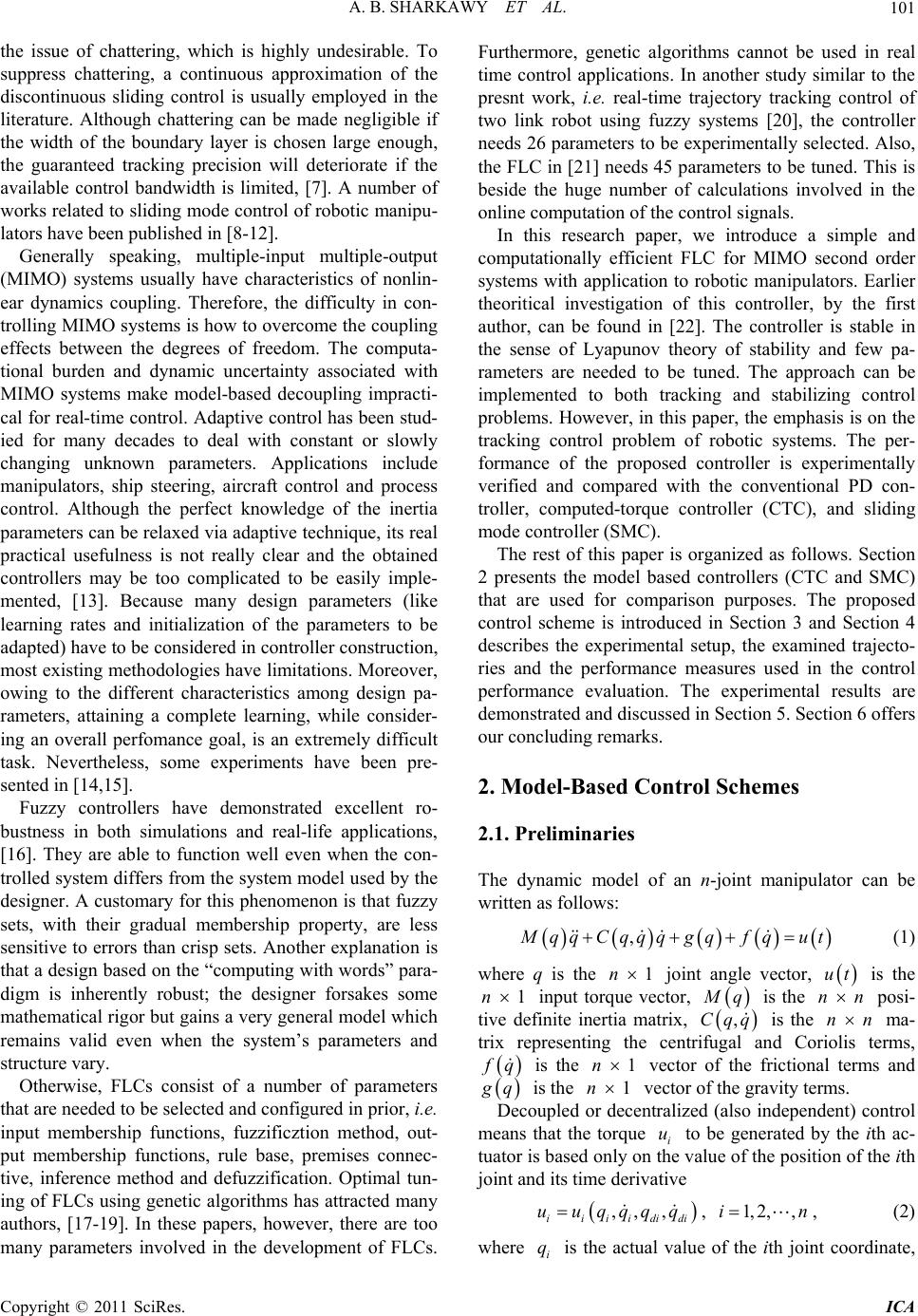

A. B. SHARKAWY ET AL.101
the issue of chattering, which is highly undesirable. To
suppress chattering, a continuous approximation of the
discontinuous sliding control is usually employed in the
literature. Although chattering can be made negligible if
the width of the boundary layer is chosen large enough,
the guaranteed tracking precision will deteriorate if the
available control bandwidth is limited, [7]. A number of
works related to sliding mode control of robotic manipu-
lators have been published in [8-12].
Generally speaking, multiple-input multiple-output
(MIMO) systems usually have characteristics of nonlin-
ear dynamics coupling. Therefore, the difficulty in con-
trolling MIMO systems is how to overcome the coupling
effects between the degrees of freedom. The computa-
tional burden and dynamic uncertainty associated with
MIMO systems make model-based decoupling impracti-
cal for real-time control. Adaptive control has been stud-
ied for many decades to deal with constant or slowly
changing unknown parameters. Applications include
manipulators, ship steering, aircraft control and process
control. Although the perfect knowledge of the inertia
parameters can be relaxed via adaptive technique, its real
practical usefulness is not really clear and the obtained
controllers may be too complicated to be easily imple-
mented, [13]. Because many design parameters (like
learning rates and initialization of the parameters to be
adapted) have to be considered in controller construction,
most existing methodologies have limitations. Moreover,
owing to the different characteristics among design pa-
rameters, attaining a complete learning, while consider-
ing an overall perfomance goal, is an extremely difficult
task. Nevertheless, some experiments have been pre-
sented in [14,15].
Fuzzy controllers have demonstrated excellent ro-
bustness in both simulations and real-life applications,
[16]. They are able to function well even when the con-
trolled system differs from the system model used by the
designer. A customary for this phenomenon is that fuzzy
sets, with their gradual membership property, are less
sensitive to errors than crisp sets. Another explanation is
that a design based on the “computing with words” para-
digm is inherently robust; the designer forsakes some
mathematical rigor but gains a very general model which
remains valid even when the system’s parameters and
structure vary.
Otherwise, FLCs consist of a number of parameters
that are needed to be selected and configured in prior, i.e.
input membership functions, fuzzificztion method, out-
put membership functions, rule base, premises connec-
tive, inference method and defuzzification. Optimal tun-
ing of FLCs using genetic algorithms has attracted many
authors, [17-19]. In these papers, however, there are too
many parameters involved in the development of FLCs.
Furthermore, genetic algorithms cannot be used in real
time control applications. In another study similar to the
presnt work, i.e. real-time trajectory tracking control of
two link robot using fuzzy systems [20], the controller
needs 26 parameters to be experimentally selected. Also,
the FLC in [21] needs 45 parameters to be tuned. This is
beside the huge number of calculations involved in the
online computation of the control signals.
In this research paper, we introduce a simple and
computationally efficient FLC for MIMO second order
systems with application to robotic manipulators. Earlier
theoritical investigation of this controller, by the first
author, can be found in [22]. The controller is stable in
the sense of Lyapunov theory of stability and few pa-
rameters are needed to be tuned. The approach can be
implemented to both tracking and stabilizing control
problems. However, in this paper, the emphasis is on the
tracking control problem of robotic systems. The per-
formance of the proposed controller is experimentally
verified and compared with the conventional PD con-
troller, computed-torque controller (CTC), and sliding
mode controller (SMC).
The rest of this paper is organized as follows. Section
2 presents the model based controllers (CTC and SMC)
that are used for comparison purposes. The proposed
control scheme is introduced in Section 3 and Section 4
describes the experimental setup, the examined trajecto-
ries and the performance measures used in the control
performance evaluation. The experimental results are
demonstrated and discussed in Section 5. Section 6 offers
our concluding remarks.
2. Model-Based Control Schemes
2.1. Preliminaries
The dynamic model of an n-joint manipulator can be
written as follows:




,

M
qqCqqqgqf qut
  (1)
where q is the 1n

joint angle vector,


ut is the
1n

input torque vector,

M
q is the nn

posi-
tive definite inertia matrix, is the

,Cqq


nn

ma-
trix representing the centrifugal and Coriolis terms,


f
q
 is the 1n

vector of the frictional terms and


g
q is the 1n

vector of the gravity terms.
Decoupled or decentralized (also independent) control
means that the torque i to be generated by the ith ac-
tuator is based only on the value of the position of the ith
joint and its time derivative
u


,, ,
iii i di di
uuqqqq , , (2) 1, 2,,in
where is the actual value of the ith joint coordinate,
i
q

A. B. SHARKAWY ET AL. 102
i
and di is its desired value. The later (di ) is usually
available signal from the robot operating system and is
planned in advance. Generally, defining the position er-
ror as , (2) can be written as
q q
n
idi
eq q
ii
uu
where, again, d
eq q

 is the difference between the
desired joint position vector and the actual one.
Obviously, the assumption of exact knowledge of the
robot dynamic model cannot be satisfied in practical
cases. Hence, the achievement of the desired tracking
performance cannot be guaranteed. For this purpose, it
would be desirable to add a term in the controller that
compensates for the modeling errors. Several related
works can be found in literature which suggests the use
of neural networks [23] and neuro-fuzzy systems [24]
in-order to compensate for the modeling errors. However,
a complete review in this area is out of the scope of this
work. In the experimental verification (Section 5), the
CTC algorithm has been implemented as it is shown in
Figure 1.

,
ii
ee
, 1,2,,i

 (3)
This approach is widely adopted in industrial settings
because of its simplicity (no dynamic model is required,
in general) and because of its fault-tolerant feature, since,
in case a single joint is affected by a failure, the robot
can be retrieved in a safe position by means of the other
joints.
The motion control problem of manipulators in joint
space can be stated in the following terms. Assume that
the joint position q and the joint velocity q are available
for measurement. Let the desired joint position d be a
differential vector function. We define a motion control-
ler as a controller which determines the actuator torques
u in such a way that the following control aim be
achieved:
q
2.3. Sliding Mode Control
In this subsection, the well-developed literature is used to
demonstrate the main features and assumptions needed to
synthesis a SMC for robotic systems. SMC employs a
discontinuous control effort to derive the system trajec-
tories toward a sliding surface, and then switching on
that surface. Accordingly, it will gradually approach the
control objectives, i.e. keep these trajectories at the ori-
gin of the phase plane. The following assumptions are
needed to synthesis a SMC.
 
lim d
tqtq t   (4)
2.2. Computed Torque Control
The computed torque (also called inverse dynamics)
technique is a special application of feedback lineariza-
tion of nonlinear systems. The computed torque control-
ler is utilized to linearize the nonlinear equation of robot
motion by cancellation of some, or all, nonlinear terms.
For this purpose, the dynamic model of the manipulator
is exploited. Taking into account (1) and defining
Assumption 1: The matrix

M
q is positive definite
and is bounded by a known positive definite matrix


ˆ
M
q.
Assumption 2: There exists a known estimate


ˆ,hqq

for the vector function


,hqq
 in (5).
Now, let us define the linear time-varying surface


s
t, [9]:

hqq
 
,,Cqqq gqf


q

(5)




 
T
12
,
,,,
n
st ett
s
tststst
 







(7)
we can derive the control scheme shown in Figure 1,
where
p
K
and v
K
are user-chosen diagonal matrices.
So that the system is decoupled, linearized and the error
dynamics is governed by the following expression [23]: where


t 
is a time-varying linear function.
From (1), (5) and (7), we can get the equivalent con-
troller (also called ideal controller)
0
vp
eKeKe 
  (6)
Robot
)(qM
),( qqh
v
K
p
K
q
q

d
q
d
q

d
q

_
_
+
+
u
Figure 1. Computed torque control scheme.

A. B. SHARKAWY ET AL. 103
 
,)
eq d
ut hqqMqq


 





(8)
where


eq
ut is equivalently the average value of


ut
which maintains the system’s trajectories (i.e. tracking
errors) on the sliding surface . To ensure that
they attain the sliding surface in a finite time and there-
after maintain there, the control torque

0st 


ut consists of
a low frequency (average) component


eq
ut and a
hitting (high frequency) component


ht
ut so that:
 
eq ht
ututu t (9)
The role of


ht
ut acts to overcome the effects of the
uncertainties and bends the entire system trajectories
towards the sliding surface until sliding mode occurs.
The hitting controller


ht
ut
is taken as:
 
sgn
ht
ut MqKs (10)
where


12
diag,,n
K
kk k
 
12
sgn ,sgn,sss

 
, , and
.
0
i
k

,sgn n
1, 2,in
T
s

sgn 

To verify the control stability, let us first get an ex-
pression for


s
t
. Using (1), (5), (9) and (10), the first
derivative of (7) is:
 
 
 


1
1
,
,
sgn
d
d
ht
sqtett
qt qtt
q tMquthqqt
Mqu
Ks







 






 

 (11)
Choosing a Lyapunov function

2
1
1
2
n
si
i
Vs

t (12)
and differentiating (12) using (11)
  

11
1
sgn
0.
nn
siiii i
ii
n
ii
i
Vstst kstst
kst



 



(13)
which provides an asymptotically stable system.
Since the parameters of (1) and (5) depend on the ma-
nipulator structure, it is difficult to obtain completely
accurate values for

M
q and . In SMC theory,
estimated values are usually used in the control context
instead of the exact parameters. So that, (8)-(10) can be
written as:

,hqq


,
 
 
 
ˆˆ
,
ˆsgn ,
eq d
ht
eq ht
ut hqqMqq
ut MqKs
ututu t


 





(14)
where

ˆ
M
q and are bounded estimates for

ˆ,hqq



M
q and


,qq
tively. As mentioned earlier
mption2, they are assumed to be known in
advance.
In sliding
h
1 and
mode, th
respec
e system trajectories are governed
in assu
by:


i
st 0

and


0
i
st
, 1,2,,in (15)
at, thynamicsre determinSo th
funct
e error d aed by the
ion


t  . If the coefficients of

t  were cho-
sen to corresnd to the coefficients of itz polyno-
mial, it is thus implying that

lim 0
tet  . This sug-
gests
po Hurw


t  taking the following form:






12
dcetcett
 with t

12
,0cc (16)
at ing mode, the error dynamics is: So th the slidin




12
0et cetcet


 , (17)
e desirmance is gover
iding mode controller in (14) can
PrFLC Scheme
apued Fuzzy Logic Controllers
sectipply the fuzzy synthesis [25], to the
and th
gu
. The
.1. Ly
this
red perfo
th
oposed
nov Bas
on, we a
ned by the coeffi-
cients 1 c and 2 c.
In sumary, e slm
arantee the stability in the Lyapunov sense even under
parameter variations. As a result, the system trajectories
are confining to the sliding surfaces (7). The control law
(14) however, shows that the coupling effects have not
been eliminated since the control signal for each degree
of freedom is dependent on the dynamics of the other
degrees of freedom. Independency is usually preferred in
practice. Furthermore, to satisfy the existence condition
of the sliding modes, a large uncertainty bound should be
used. In this case, the controller results in large imple-
mentation cost and may lead to chattering efforts which
should be avoided in practical implementation.
3
3
In
design of stable controllers. To this end, consider a class
of MIMO nonlinear second order systems whose dy-
namic equation can be expressed as:




,,
x
tfxxu  , (18)
where


,,
f
xxu
 is an
inpu
continuous function, u unknown
is the cot and ntrol


12 T
11 1
,,,
n
x
txx x

  is the state
vector and T
12
22 2
,,,
n
xx xx
dx
dt





, wher
e 12
ii
x
x

,
1, 2,,in

. apunov We now seek a smooth Lyfunction
n
:VR
that is po
n
R
sitiv
for the continuous feedback model (18)
e definite, i.e.

0Vx when 0x

and


0Vx

when x = 0, and gfinity: rows to in


x
general
V
as T xx. Obviously, tfor a his holds ized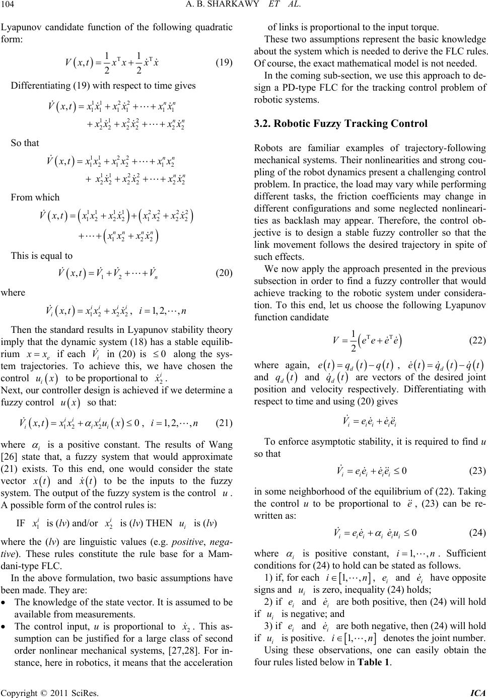

A. B. SHARKAWY ET AL. 104
Lyapunovg quadrati
:
candidate function of the followin
form
c

TT
11
,22 Vxtxx xx
 (19)
Differentiating (19) with respect to time gives

1122
11111 1
,nn Vxtxx xxxx
11 22
22 2222
nn
x
xxxxx


 
 


So that

112 2
121 212
11 22
22 2222
,
nn
nn
Vxtxx xxxx
x
xxxxx






From which

This is equal to

(20)
where
Then the standard results in unov stability theory
imply that the dynamic system (18) has a stabuilib-
riu

,Vxt


111122 22
12221 222
12 22
nn nn
xx xxxxxx
xx xx

 




12
,n VxtV VV



12 22
,iiii
i
Vxtxx xx
, 1, 2,,in
Lyap
le eq
m e
x
x if each i V
 in (20) is 0 along the sys-
tem trajectories. To achieve this, we have chosen the
contro

ix to be pportional to 2
l

uro i
x
.
Next, our controller design is achieved if we determine a
fuzzy co

ux so that: ntrol
where
 
2
,0
iii
iii
Vxt xux   
, 1,2,,in (21)
12
xx 
i

ists
is a positive constant. The results o
[26] state that, a fuzzy system that would approximate
f Wang
(21) ex. To this end, one would consider the state
vector

x
t and

x
t  to be the inputs to the fuzzy
system. The output of the fuzzy system is the control u.
A possiorm of ontrol rules is:
IF 1
i
ble fthe c
x
is (lv) and/or 2
i
x
is (lv) THEN u is (lv)
i
whe sti os a-
tive hetut-
are:

surements.
re the (lv) are linguic values (e.g. p itive, neg
). Tse rules constie the rule base for a Mam
dani-type FLC.
In the above formulation, two basic assumptions have
been made. They
The knowledge of the state vector. It is assumed to be
available from mea
 The control input, u is proportional to 2
x
. This as-
sumption can be justified for a largf second
rules.
O
ro
zy Tracking Control
ry-following
echanical systems. Their nonlinearities and strong cou-
rder to find a fuzzy controller that would
ac
e class o
order nonlinear mechanical systems, [27,28]. For in-
stance, here in robotics, it means that the acceleration
of links is proportional to the input torque.
These two assumptions represent the basic knowledge
about the system which is needed to derive the FLC
f course, the exact mathematical model is not needed.
In the coming sub-section, we use this approach to de-
sign a PD-type FLC for the tracking control problem of
botic systems.
3.2. Robotic Fuz
Robots are familiar examples of trajecto
m
pling of the robot dynamics present a challenging control
problem. In practice, the load may vary while performing
different tasks, the friction coefficients may change in
different configurations and some neglected nonlineari-
ties as backlash may appear. Therefore, the control ob-
jective is to design a stable fuzzy controller so that the
link movement follows the desired trajectory in spite of
such effects.
We now apply the approach presented in the previous
subsection in o
hieve tracking to the robotic system under considera-
tion. To this end, let us choose the following Lyapunov
function candidate

TT
1
Ve
2eee
 (22)
where again,




d
etq tqt

,





d
etq tqt
 


d
qt and and


d
qt
 are vectors
locity respectiv
of the desired joint
ely. Differentiating withposition and ve
respeime andg (20) gives
iiiii
Veeee

ct to t usin
To enforce asymptotic stability, it is required to find u
so that
0Veeee
iiiii


 (23)
in some neighborhood of the equilibr
the control u to be proportional to
ium of (22). Taking
, (23) can be re- e

written as:
0
iiiiii
Vee eu 


 (24)
where i

is positive constant,
(24) to hold can
fo
1,i
be stated as
,n. Sufficient
follows. conditions for
1) if, r each


1, ,in, i e aave opposite
signs and i u is zero, inequality (24) holds;
nd h i e 
2) if i e and i epositive, then (24) will hold
if i u is negative; and
 are both
3) if i and i e are both negative, then (24) will hold
if is positive.
e
i
u


1 , ,indenotes the joint number.
ow in Tab
Using these observations, one can easily obtain the
four rules listed belle 1.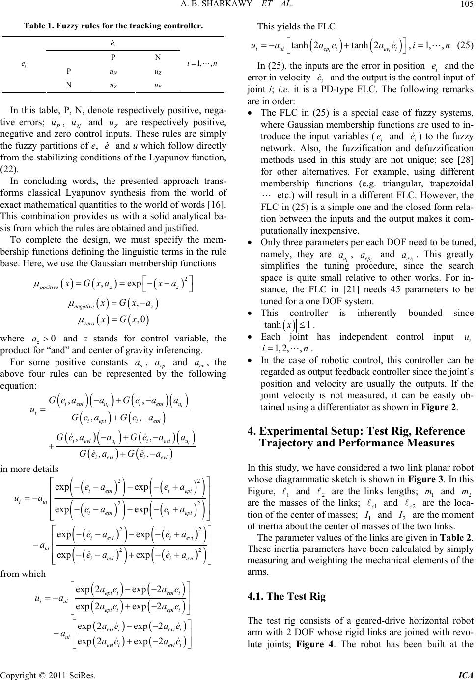

A. B. SHARKAWY ET AL.105
Table 1. Fuzzy rules for the tracking controller.
i
e

P N
P uNu
Z
i
e
N uZ u
P
1, ,in


In this table, , denoespectiv positive, nega-
ve errors;
P, Nte rely
ti
P
u,
N
u and
Z
u
a
are respectively positive,
ne
lassical Lyapunov synthesis from the world
ex
rule
ba
gative and zero control inputs. These rules are simply
the fuzzy paronf e, e
nd u which follow directly
from the stabilizing conditions of the Lyapunov function,
(22).
In concluding words, the presented approach trans-
forms c
titis o
of
act mathematical quantities to the world of words [16].
This combination provides us with a solid analytical ba-
sis from which the rules are obtained and justified.
To complete the design, we must specify the mem-
bership functions defining the linguistic terms in the
se. Here, we use the Gaussian membership functions
 
2
,exp
positive zz
xGxa xa 



 
,
negative z
x
Gx a  
 
,0
zero
x
Gx  
where and z stands for control variable, the
product nd” and center of gravity inferencing.
some p
in
eq
0
z
a
for “a
g
For ositive constants u a, ep a and ev a, the
above four rules can be represented by the follow
uation:




 




 
,,
ii
iepiuiepi u
i
GeaaGe aa
u  ,,
,,
,,
ii
iepii epi
i eviuieviu
i eviievi
GeaGe a
GeaaGeaa
GeaGe a

 



in more details















 
2
2
22
2
2
2
2
p exp
exp exp
exp exp
exp exp
i epii epi
iui
i epii epi
i evii evi
ui
i eviievi
ea ea
ea ea
ea ea
aea ea









 




from which


ex
ua

 











exp 2exp2
exp 2exp2
exp 2exp2
exp 2exp2
epi iepi i
i
uu
i
epiiepii
evi ievi i
ui evi ievi i
ae ae
aae ae
ae ae
aae ae














This yields the FLC


tanh 2tanh 2
ii
iuiepievi
ua aeae



 


,1,,
in (25)
In (25), the inputs are the error in position and the
error in velocity and the output is the contrl input of
joint i; i.e. it is a PD-type FLC. The followinremarks
ar
 The FLC in (25) is a special case of fuzzy sy
where Gaussian membership functions are used t
t
,
natives. For e amng different
.
i
e
o
g
i
e

e in order:
stems,
o in-
troduce the input variables (i e and i e
) tohe fuzzy
network. Alsothe fuzzification and defuzzification
methods used in this study are not unique; see [28]
for other alterxple, usi
membership functions (e.g. triangular, trapezoidal
 etc.) will result in a different FLC. However, the
FLC in (25) is a simple one and the closed form rela-
tion between the inputs and the output makes it com-
putationally inexpensive.
 Only three parameters per each DOF need to be tuned,
namely, they are i
u
a, i
ep
a and i
ev
a. This greatly
simplifies the tuning procedure, since the search
space is quite small relative to other works. For in-
stance, the FLC in [21] needs 45 parameters to be
tuned for a one DOF system
 This controller is inherently bounded since


tanh 1x

.
 Each joint has independent control input i u
1, 2,,in

.
 In the case of robotic control, this controller can be
regarded as output feedback controller since the joint’s
joi easured, it can be easily ob-
igure, and are the links lengths; and
tio
position and velocity are usually the outputs. If the
nt velocity is not m
tained using a differentiator as shown in Figure 2.
4. Experimental Setup: Test Rig, Reference
Trajectory and Per formance Measures
In this study, we have considered a two link planar robot
whose diagrammatic sketch is shown in Figure 3. In this
F1 212
are the masses of the links; 1c  and 2c  are the loca
n of the center of masses; 1
 mm
-
I
and 2
I
are the moment
of inertioutnter ofks.
ments of the
ints; Figure 4. The robot has been built at the
a ab the ce masses of the two lin
The parameter values of the links are given in Table 2.
These inertia parameters have been calculated by simply
measuring and weighting the mechanical ele
arms.
4.1. The Test Rig
The test rig consists of a geared-drive horizontal robot
arm with 2 DOF whose rigid links are joined with revo-
lute jo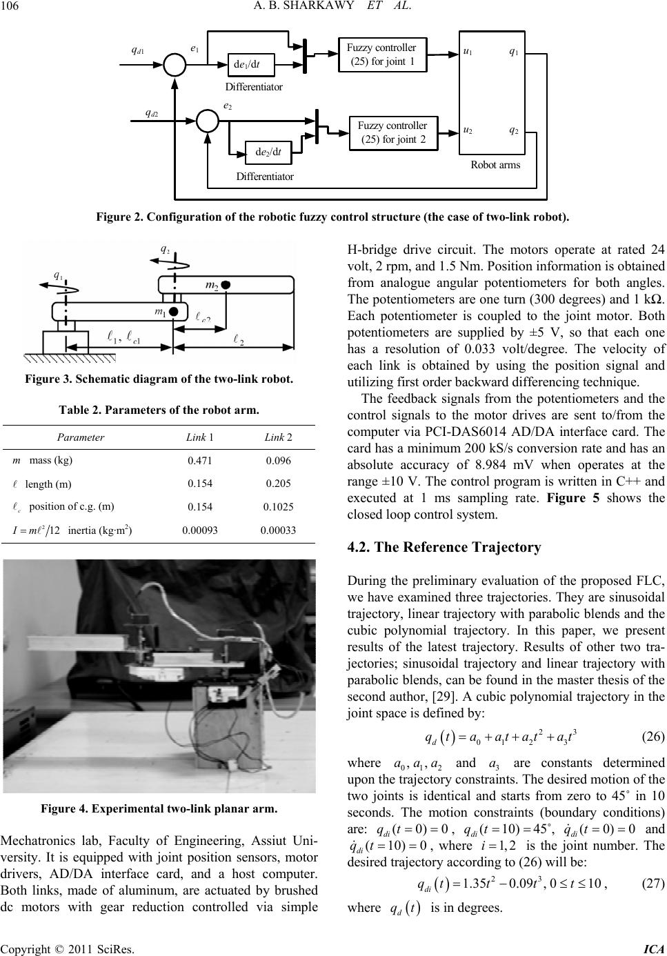

A. B. SHARKAWY ET AL. 106
Fuzzy controller
(25) for joint 1
Fuzzy controller
(25) for joint 2
2d
q
2
q
1d
q
2
u
Robot arms
1
q
1
u
dtde /
1
dtde /
2
1
e
2
e
Differentiator
Differentiator
de
1
/dt
de
2
/dt
e
1
q
d1
q
d2
q
1
u
1
e
2
q
2
u
2
Figure 2. Configuration of the robotic fuzzy control structure (the case of two-link robot).
Figure 3. Schematic diagram of the two-link r obot.
Table 2. Parameters of the robot arm.
Parameter Link 1 Link 2
m mass (0.096 kg) 0.471
 length
.g. (m)
(m) 0.154 0.205
c
 position of c0.154 0.1025
212m ineIrtia (kg·m2) 0 0 .00093.00033
Figure 4. Experimental two-link planar arm.
Mechatronics lab, Faculty of Engineering, Assiut Uni
versity motor
rivers, AD/DA interface card, and a host computer.
H-bridge drive circuit. The motors operate at rated 24
n is obtained
from analogue angular potentiometers for both angles.
d
ex
blends and the
ubic polynomial trajectory. In this paper, we present
lts of other two tra-
ctories; sinusoidal trajectory and linear trajectory with
-
volt, 2 rpm, and 1.5 Nm. Position informatio
. It is equipped with joint position sensors,
d
Both links, made of aluminum, are actuated by brushed
dc motors with gear reduction controlled via simple
The potentiometers are one turn (300 degrees) and 1 kΩ.
Each potentiometer is coupled to the joint motor. Both
potentiometers are supplied by ±5 V, so that each one
has a resolution of 0.033 volt/degree. The velocity of
each link is obtained by using the position signal and
utilizing first order backward differencing technique.
The feedback signals from the potentiometers and the
control signals to the motor drives are sent to/from the
computer via PCI-DAS6014 AD/DA interface card. The
card has a minimum 200 kS/s conversion rate and has an
absolute accuracy of 8.984 mV when operates at the
range ±10 V. The control program is written in C++ an
ecuted at 1 ms sampling rate. Figure 5 shows the
closed loop control system.
4.2. The Reference Trajectory
During the preliminary evaluation of the proposed FLC,
we have examined three trajectories. They are sinusoidal
trajectory, linear trajectory with parabolic
c
results of the latest trajectory. Resu
je
parabolic blends, can be found in the master thesis of the
second author, [29]. A cubic polynomial trajectory in the
joint space is defined by:


23
01 23 d
qtaatatat (26)
where 012
,,aaa and 3 a are constants determined
upon the trajectory constraints. The desired motion of the
two joints is identical and starts from zero to 45˚ in 10
seconds. The motion constraints (boundary conditions)
are: (0)qt 0
di

, ( 10)
di
qt

45˚, (0)0 and
di
qt

(10)0
di
qt

, w
here 21,i

is the joint number. The
desiredto (26) will be: trajectory according


23
1.350.09, 010
di
qttt t

, (27)
where


d
qt is in degrees.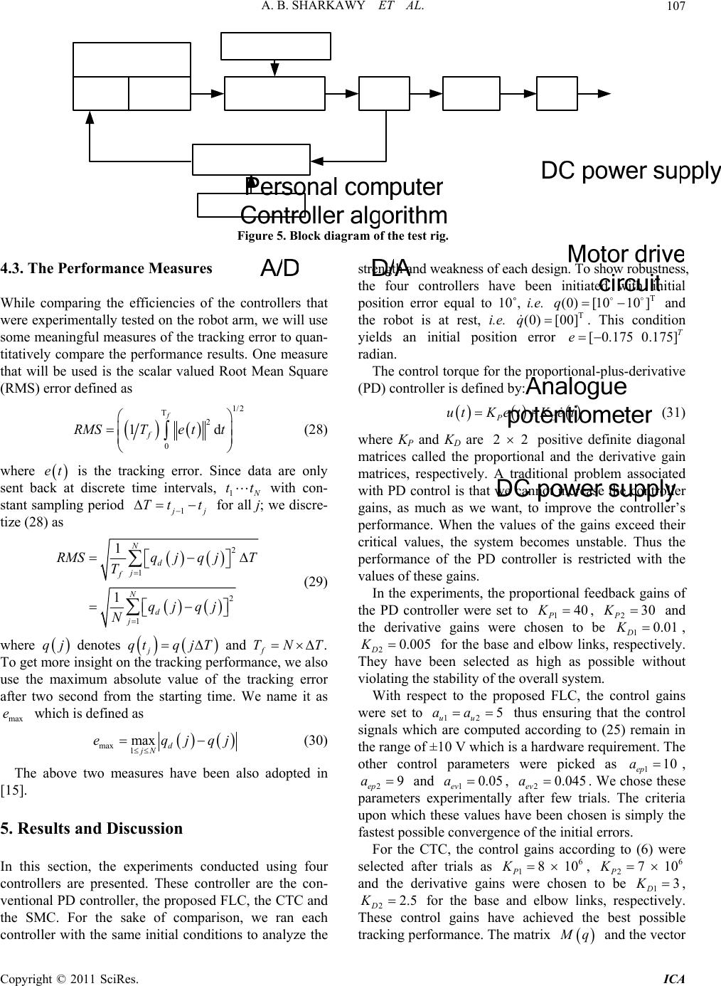

A. B. SHARKAWY ET AL.107
Figure 5. Block diagram of the test rig.
4.3. The Performance Measures
While comparing the efficiencies of the
ere experimentally tested on the robot arm, we will use
king error to quan-
tatively compare the performance results. One measure
controllers that
w
some meaningful measures of the trac
ti
that will be used is the scalar valued Root Mean Square
(RMS) error defined as


1/2
T
2
0
1d
f
f
RMSTe tt




 (28)
where is the tracking error. Since data are only
discrete time intervals,

et
sent back at 1
N
tt with con-
stant samling period p1
j
j
Ttt

  for all j; we discre-
tize (28) as
 
 
2
1
2
1
1N
d
j
T
qjqj
N






where
1N
d
j
f
RMSqjqj
T



(29)


qj denotes



j
qtq jT and fNTT

 .
To get mnsight oform
use the maximum absolute value of the tracking error
after two second from the starting time. We name it as
as
ore in the tracking perance, we also
max
e which is defined


max 1
max d
jN
eqjqj

 (30)
The above two measures have been also adopted in
[15].
5. Results a
n, the experiments conducted using four
are the con-
osed FLC, the CTC and
e SMC. For the sake of comparison, we ran each
strength and weakness of each design. To show robustness,
the four controllers have been initiated with initial
ual to 10˚, i.e. T (0)[1010 ]q

and
the robot is at rest, i.e. . This condition
nd Discussion
n this sectioI
controllers are presented. These controller
ventional PD controller, the prop
th
controller with the same initial conditions to analyze the
yields an initial position error [0.175 0.175]T
e
radian.
The control torque for the proportional-plus-derivative
(PD) controller is defined by:
position error eq
T
(0)[00]q





PD
utKet Ket  (31)
where KP and KD are 2 2

pogonal
matrices called the propore derivative gain
matrices, respectively. A traditional
with PD c
sitive definite dia
tional and th
problem associated
ontrol is that we cannot increase the controller
ga
of the gains exceed their
critical values, the system becomes u
performance of the PD controller is restri
ins, as much as we want, to improve the controller’s
performance. When the values
nstable. Thus the
cted with the
values of these gains.
In the experiments, the proportional feedback gains of
the PD controller were set to 140
P
K, 230
P
K

and
the derivative gains were chosen to be 10.01
D
K

,
20.005 D
K

for the base and elbow links, respectively.
They have been selected as high as possible without
violating the stability of the overall system.
With respect to the proposed FLC, the control gains
were set to 12uu aa5

 thus ensuring that the control
sig
ardware uirement
nals which are computed according to (25) remain in
the range of ±10 V which is a hreq. The
other control parameters were picked as110
ep
a

,
29 ep
a

and 10.05
ev
a

, 20.045
ev
a. We chose these
parameters experimentally after few trials. The criteria
upon which these values have been chosen is simply the
fa
C, the cont
stest possible convergence of the initial errors.
For the CTrol gains according to (6) were
selected after trials as 6
18 10 P
K , 6
27 10 P
K
and the derivative gains were chosen to be 13
D
K

,
22.5 D
K

for the base and elbow links, respectively.
ontrolve e best possible
tracking performance. The matrix

These c gains haachieved th
M
q and the vector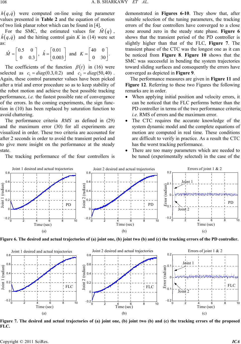

A. B. SHARKAWY ET AL. 108
otion
stimated values for

,hqq
 were computed on-line using the parameter
values presented in Table 2 and the equation of m
of two link planar robot which can be found in [4].
For the SMC, the e


ˆ
M
q
ere se
,

ˆ,
hqq
 and the hitting control gain K in (14) wt
0.5 0
ˆ
00.3
M 

, 0.01
ˆ
0.003
h 

a40 0
030



.
The coefficients of the function

as:
nd K

t 
in (16) were
selected as 1(0.3,0.2)cdiag and 2(50, 4cdiag0)
picked
.
otion and achieve the best possible tracking
nce, i.e. the fastest possible rate of converg
rors. In thcoming expts, the sign fu
(10) has been replaced by saturation function t
mance criteria defined in (29)
Ag
after a t
robot m
performa
of the er
tion in
av
ain, these control parameter values have been
rial and error procedure so as to keep stability of
the
ence
-
o
 When applying initial position and velocity errors, it
can be noticed that the FLC performs better than the
PD controller in terms of the two performance criteria;
i.e. RMS of errors and the maximum error.
e erimennc
oid chattering.
The perforMS as
and the maximum error (30) for all experiments are
visualized in order. These two criteria are accounted for
after 2 seconds in order to avoid the transient period and
to give more insight on the performance at the steady
state.
The tracking performance of the four controllers is
R

demonstrated in Figures 6-10. They show that, after
suitable selection of the tuning parameters, the tracking
errors of the four controllers have converged to a close
zone around zero in the steady state phase. Figure 6
shows that the transient period of the PD controller is
slightly higher than that of the FLC, Figure 7. The
transient phase of the CTC was the longest one as it can
be noticed from Figure 8. Figure 10 shows that the
SMC was successful in bending the system trajectories
toward sliding surfaces and consequently the errors have
converged as depicted in Figure 9.
The performance measures are given in Figure 11 and
Figure 12. Referring to these two Figures the following
remarks are in order.
 The CTC requires the accurate knowledge of the
system dynamic model and the complete equations of
motion are computed in real time. These conditions
are difficult to verify in practice. As a result the CTC
has the worst tracking performance.
There are too many parameters which are needed to
be tuned (experimentally selected) in the case of the
Time (sec)
J
o
i
n
t
1
(
r
a
d
i
a
n
)
Joint 1 desired and actual trajectories
02468 10
-0.2
0
0. 2
0. 4
0. 6
0. 8
PD
Time (sec)
J
d actual trajectories
-
oint 2(radian)
Joint 2 desired an
02 46 810
-0.2
0
0.2
0.4
0.6
0.8
Time (sec)
E
r
r
o
r
(
r
a
d
i
an)
Errors of joint 1 & 2
02468 10
-0.2
-0.1
0
0.1
0.2
Joint 1
Joint 2
PD
-
-
PD
-
(a) (b) (c)
Figure 6. The desired and actual trajectories of (a) joint one, (b) joint two (b) and (c) the tracking errors of the PD controller.
Time (sec)
t 1 (radian)
Joint 1 desired and actual trajectories
Join
02468 10
-0.2
0
0.2
0.4
0.6
0.8
FLC
Time
(
sec
)
-
Joint 2 (radian)
Joint 2 desired and actual trajectories
02 46 810
-0.2
0
0.2
0.4
0.6
0.8
FLC
Time (sec)
-
E
r
r
o
r
(
r
a
d
i
an)
Errors of joint 1 & 2
02 46 810
-0.2
0.2
-0.1
0
Joint 1
Joint 2
0.1
FLC
-
-
(a) (b) (c)
Figure 7. The desired and actual trajectories of (a) joint one, (b) joint two (b) and (c) the tracking errors of the proposed
FLC.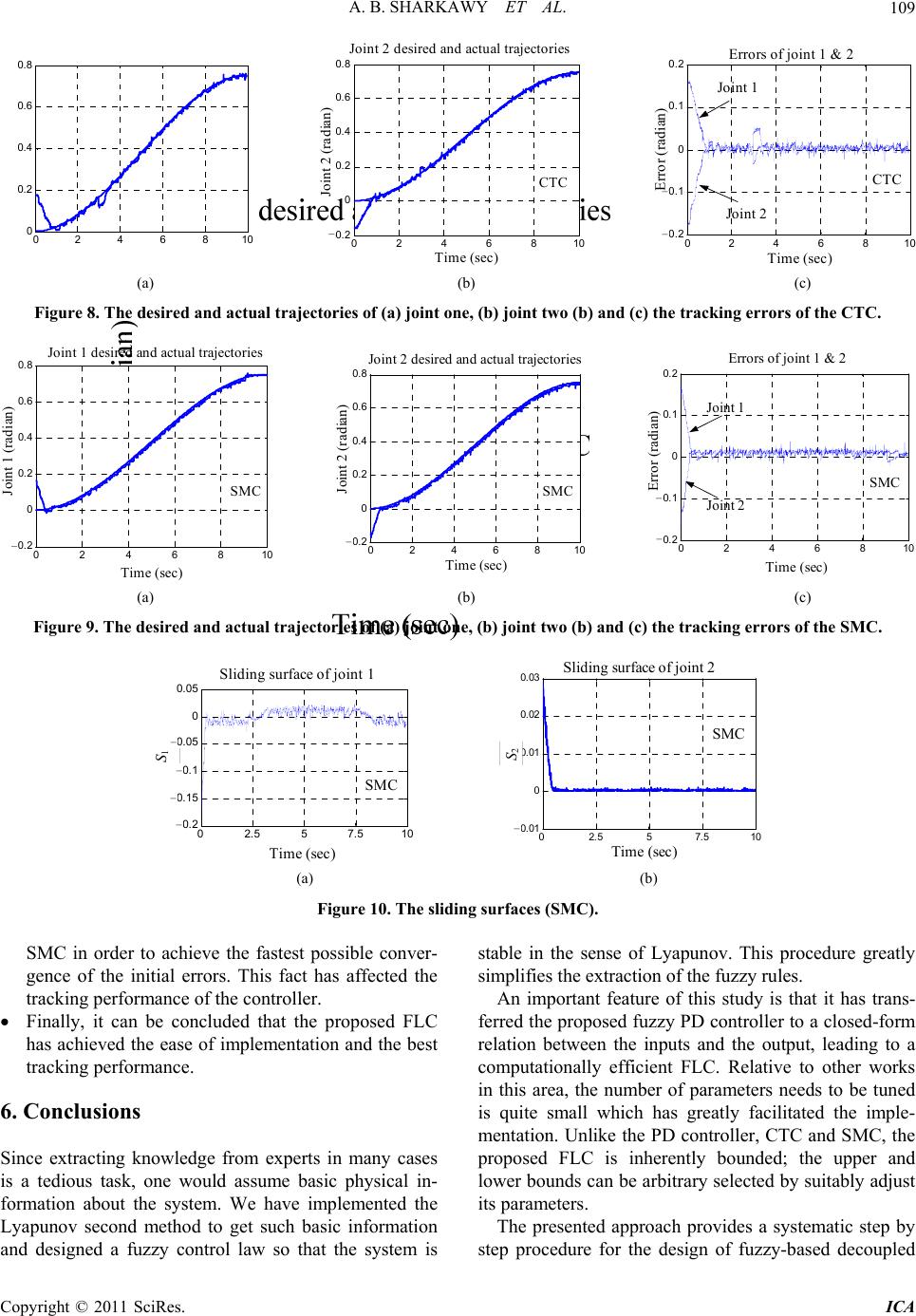

A. B. SHARKAWY ET AL.109
Joint 2 desired and actual trajectories
Time (sec)
02 4 6 810
0
0.2
0.4
0.6
0.8
J
o
i
n
t
2
(
r
a
d
i
a
n
)
0 2 4 6 810
-0.2
0
0.2
0.4
0.6
0.8
CTC
-
Errors of joint 1 & 2
Time (sec)
Error (radian)
02 4 6 81
0
-0.2
-0.1
0
0.1
0.2
Joint 1
Joint 2
CTC
-
-
(a)c)
Joint 1 desired and actual trajectorie
(b) (
Figure 8. The desired and actual trajectories of (a) joint one, (b) joint two (b) and (c) the tracking errors of the CTC.
s
Time (sec)
J
o
i
nt
1
(
r
a
d
i
an)
0 2 46 810
-0.2
0
0. 2
0. 4
0. 6
0. 8
SMC
-
Joint 2 desired and actual trajectories
Time (sec)
Joint 2 (radian)
0246810
-0. 2
0
0.2
0.4
0.6
0.8
SMC
-
0 24 6810
-0.2
-0.1
0
0.1
0.2 Errors of joint 1 & 2
Time (sec)
E
r
r
o
r
(
r
a
d
i
a
n
)
Joint 1
Joint 2
SMC
-
-
(a) (b) (c)
Figure 9. The desired and actual trajectories of (a) joint one, (b) joint two (b) and (c) the tracking errors of the SMC.
Sliding surface of joint
1
Time (sec)
0 2.5 57.5 10
-0. 2
-0.15
-0. 1
-0.05
0
0. 05
SMC
-
-
-
-
S
1
Sliding surface of joint 2
Time (sec)
0 2.557.5 10
-0.01
0
0.01
0.02
0.03
SMC
S
2
-
(a) (b )
SM
gence of the initial errors. This fact has affected the
tracking performance of the controller.
 Finally, it can be concluded that the proposed FLC
has achieved the ease of implementation and the best
tracking performance.
6. Conclusions
Since extracting knowledge from experts in many ca
is a tedious task, one would assume
formation about the system. We have im
apunov second method to get such b
nd designed a fuzzy control law so that the system is
simplifies the extraction of the fuzzy rules.
An important feature of this study is that it has trans-
ferred the proposed fuzzy PD controller to a closed-form
relation between the inputs and the output, leading to a
computationally efficient FLC. Relative to other works
in this area, the number of parameters needs to be tuned
is quite small which has greatly facilitated the imple-
mentation. Unlike the PD controller, CTC and SMC, the
posed FLC is inherently boundhe upper and
trary selected by suitably adjust
approach provides a systematic step by
step procedure for the design of fuzzy-based decoupled
Figure 10. The sliding surfaces (SMC).
C in order to achieve the fastest possible conver- stable in the sense of Lyapunov. This procedure greatly
ses proed; t
basic physical in- lower bounds can be arbi
plemented the
asic information
its parameters.
The presented Ly
a

A. B. SHARKAWY ET AL. 110
t 2 for the four controllers in ian. Figure 11. The RMS error of joint 1 and joinrad
Figure 12. The maximum error of the four controllers in radian.
edback controllers
rder nonlinear systems. This control scheme has been
applied to the control of a two-link robot. It can also be
extended to n number of link robots. Experimental re-
sults show that the design procedure has been successful
in representing the nonlinear dynamics in the control
context and resulted in a stable closed-loop control. Ro-
bustness of the FLC has been examined via initial posi-
tion errors. Relative to the conventional PD controller,
CTC and SMC, the proposed FLC exhibits the best per-
formance.
7. References
[1] Z. Bingul and O. Karahan, “A Fuzzy Logic Controller
Tuned with PSO for 2 D
Expert Systems with Applications, Vol. 38, No. 1, 2011,
fe
o
for a wide class of MIMO second
OF Robot Trajectory Control,”
pp. 1017-1031. doi:10.1016/j.eswa.2010.07.131
[2] T.-H. S. Li and Y.-C. Huang, “MIMO Adaptive Fuzzy
Terminal Sliding-Mode Controller for Robotic Manipu-
lators,” Information Sciences, Vol. 180, No. 23, 2010, pp.
4641-4660. doi:10.1016/j.ins.2010.08.009
[3] L. Tian and C. Collins, “Optimal Placement of a
Two-Link Planar Manipulator Using a Genetic Algo-
rithm,” Robotica, Cambridge University Press, Cam-
bridge, Vol. 23, No. 2, 2005, pp. 169-176.
[4] M. W. Spong, S. Hutchinson and M. Vidyasagar, “Robot
Modeling and Control,” John Wiley & Sons Inc., New
York, 2006.
[5] F. Reyes and R. Kelly, “Experimental Evaluation of
Model-Based Controllers on a Direct-Drive Robot Arm,”
Mechatronics, Vol. 11, No. 3, 2001, pp. 267-282.
doi:10.1016/S0957-4158(00)00008-8
[6] J. Slotine and W. Li, “Applied Nonlinear Control,” Pren-
tice-Hall Inc., New Jersey, 1991.
[7] H. B. Guo, Y. G. Liu, G. R. Liu and H. R. Li, “Cascade
Control of a Hydraulically Driven 6-DOF Parallel Robot
Manipulator Based on a Slidg Mode,” Control Engi-
, No. 9, 2008, pp. 1055-1068.
doi:10.1016/j.conengprac.2007.11.005
in
neering Practice, Vol. 16
[8] W. Gueaieb, S. Al-Sharhan and M. Bolic, “Robust Com-
Putationally Efficient Control of Cooperative Closed-
Chain Manipulators with Uncertain Dynamics,” Auto-
matica, Vol. 43, 2007, pp. 842-851.
doi:10.1016/j.automatica.2006.10.025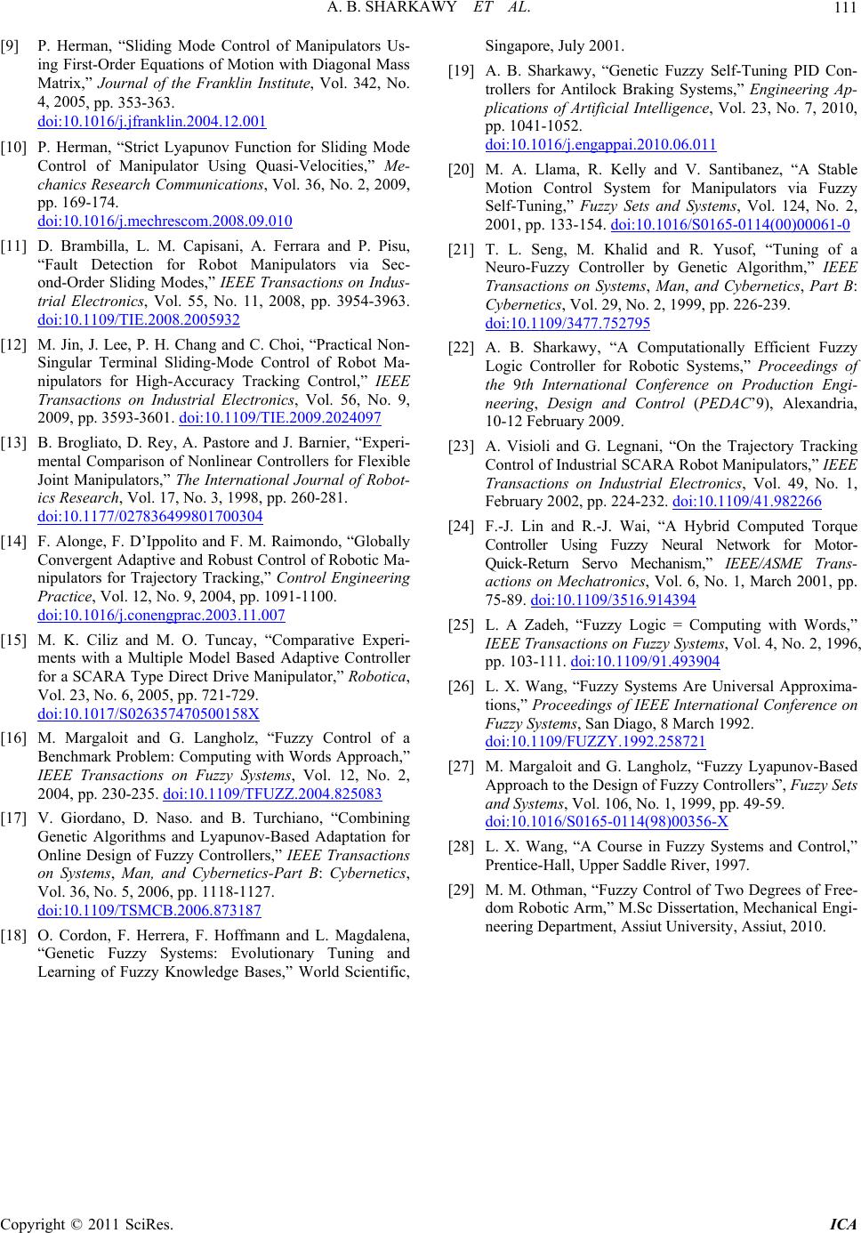

A. B. SHARKAWY ET AL.111
, pp. 353-363.
franklin.2004.12.001
[9] P. Herman, “Sliding Mode Control of Manipulators Us-
ing First-Order Equations of Motion with Diagonal Mass
Matrix,” Journal of the Franklin Institute, Vol. 342, No.
4, 2005
doi:10.1016/j.j
trict Lyapunov Function for Sliding Mode [10] P. Herman, “S
Control of Manipulator Using Quasi-Velocities,”
chanics Research Communications, Vol. 36, No. 2, 2009,
pp. 169-174.
Me-
doi:10.1016/j.mechrescom.2008.09.010
D. Brambilla, L. M. Capisani, A. Ferrara and [11] P. Pisu,
“Fault Detection for Robot Manipulators via Sec-
ond-Order Sliding Modes,” IEEE Transactions on Indus-
trial Electronics, Vol. 55, No. 11, 2008, pp. 3954-3963.
doi:10.1109/TIE.2008.2005932
[12] M. Jin, J. Lee, P. H. Chang and C. Choi, “Practical Non-
Singular Terminal Sliding-Mode Control of Robot Ma-
nipulators for High-Accuracy Tracking Control,” IEEE
Transactions on Industrial Electronics, Vol. 56, No. 9,
2009, pp. 3593-3601. doi:10.1109/TIE.2009.2024097
[13] B. Brogliato, D. Rey, A. Pastore and J. Barnier, “Experi-
mental Comparison of Nonlinear Controllers for Flexible
Joint Manipulators,” The International Journal of Robot-
ics Research, Vol. 17, No. 3, 1998, pp. 260-281.
doi:10.1177/027836499801700304
[14] F. Alonge, F. D’Ippolito and F. M. Raimondo, “Globally
Convergent Adaptive and Robust Control of Robotic Ma-
nipulators for Trajectory Tracking,” Control Engineering
Practice, Vol. 12, No. 9, 2004, pp. 1091-1100.
doi:10.1016/j.conengprac.2003.11.007
[15] M. K. Ciliz and M. O. Tuncay, “Comparative Experi-
ments with a Multiple Model Based Adaptive Controller
for a SCARA Type Direct Drive Manipulator,” Robotica,
Vol. 23, No. 6, 2005, pp. 721-729.
doi:10.1017/S026357470500158X
[16] M. Margaloit and G. Langholz, “Fuzzy Control of a
Benchmark Problem: Computing with Words Approach,”
IEEE Transactions on Fuzzy Systems
2004, pp. 230-235. doi:10.1109/TFUZZ
, Vol. 12, No. 2,
.2004.825083
Part B: Cyberne t ic s,
[17] V. Giordano, D. Naso. and B. Turchiano, “Combining
Genetic Algorithms and Lyapunov-Based Adaptation for
Online Design of Fuzzy Controllers,” IEEE Transactions
on Systems, Man, and Cybernetics-
Vol. 36, No. 5, 2006, pp. 1118-1127.
doi:10.1109/TSMCB.2006.873187
[18] O. Cordon, F. Herrera, F. Hoffmann and L. Magdalena,
“Genetic Fuzzy Systems: Evolutionary Tuning and
Learning of Fuzzy Knowledge Bases,” W
Singapore, July 2001.
[19] A. B. Sharkawy, “Genetic Fuzzy Self-Tuning PID Con-
trollers for Antilock Braking Systems,” Engineering Ap-
plications of Artificial Intelligence, Vol. 23, No. 7, 2010,
pp. 1041-1052.
doi:10.1016/j.engappai.2010.06.011
[20] M. A. Llama, R. Kelly and V. Santibanez, “A Stable
Motion Control System for Manipulators via Fuzzy
Self-Tuning,” Fuzzy Sets and Systems, Vol. 124, No. 2,
2001, pp. 133-154. doi:10.1016/S0165-0114(00)00061-0
f, “Tuning of a [21] T. L. Seng, M. Khalid and R. Yuso
Neuro-Fuzzy Controller by Genetic Algorithm,” IEEE
Transactions on Systems, Man, and Cybernetics, Part B:
Cybernetics, Vol. 29, No. 2, 1999, pp. 226-239.
doi:10.1109/3477.752795
[22] A. B. Sharkawy, “A Computationally Efficient Fuzzy
Logic Controller for Robotic Systems,” Proceedings of
the 9th International Conference on Production Engi-
neering, Design and Control (PEDAC’9), Alexandria,
10-12 February 2009.
[23] A. Visioli and G. Legnani, “On the Trajectory Tracking
Control of Industrial SCARA Robot Manipulators,” IEEE
Transactions on Industrial Electronics, Vol. 49, No. 1,
February 2002, pp. 224-232. doi:10.1109/41.982266
[24] F.-J. Lin and R.-J. Wai, “A Hybrid C
Controller Using Fuzzy Neural
omputed Torque
Network for Motor-
Quick-Return Servo Mechanism,” IEEE/ASME Trans-
actions on Mechatronics, Vol. 6, No. 1, March 2001, pp.
75-89. doi:10.1109/3516.914394
[25] L. A Zadeh, “Fuzzy Logic = Computing with Words,”
IEEE Transactions on Fuzzy Systems, Vol. 4, No. 2, 1996,
pp. 103-111. doi:10.1109/91.493904
[26] L. X. Wang, “Fuzzy Systems Are Universal Approxima-
tions,” Proceedings of IEEE International Confer
Fuzzy Systems, San Diago, 8 March 1
ence on
992.
doi:10.1109/FUZZY.1992.258721
[27] M. Margaloit and G. Langholz, “Fuzzy Lyapunov-Based
Approach to the Design of Fuzzy Controllers”, Fuzzy Sets
and Systems, Vol. 106, No. 1, 1999, pp. 49-59.
doi:10.1016/S0165-0114(98)00356-X
[28] L. X. Wang, “A Course in Fuzzy Systems and Control,”
Prentice-Hall, Upper Saddle River, 1997.
[29] M. M. Othman, “Fuzzy Control of Two Degrees of Free-
dom Robotic Arm,” M.Sc Dissertation, Mechanical Engi-
neering Department, Assiut University, Assiut, 2010.
orld Scientific,
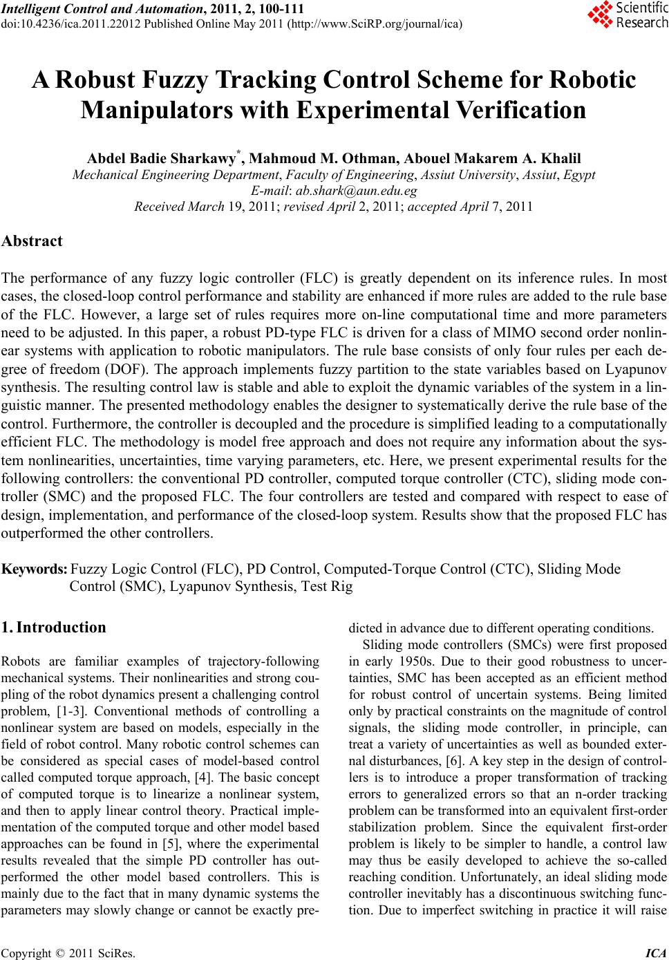