Journal of Applied Mathematics and Physics, 2014, 2, 1047-1052
Published Online November 2014 in SciRes. http://www.scirp.org/journal/jamp
http://dx.doi.org/10.4236/jamp.2014.212119
How to cite this paper: Sieniek, M., Gurgul, P. and Paszyński, M. (2014) Finite Element Method Computations of the Acous-
tics of the Human Head Based on the Projection Based Interpolation Data. Journal of Applied Mathematics and Physics, 2,
1047-1052. http://dx.doi.org/10.4236/jamp.2014.212119
Finite Element Method Computations
of the Acoustics of the Human Head
Based on the Projection Based
Interpolation Data
Marcin Sieniek, Piotr Gurgul, Maciej Paszyński
Department of Computer Science, AGH University of Science and Technology, Kraków, Poland
Received August 2014
Abstract
In this paper we present the Projection Based Interpolation (PBI) technique for construction of
continuous approximation of MRI scan data of the human head. We utilize the result of the PBI al-
gorithm to perform three dimensional (3D) Finite Element Method (FEM) simulations of the
acoustics of the human head. The computational problem is a multi-physics problem modeled as
acoustics coupled with linear elasticity. The computational grid contains tetrahedral finite ele-
ments with the number of equations and polynomial orders of approximation varying locally on
finite element edges, faces, and interiors. We utilize our own out-of-core parallel direct solver for
the solution of this multi-physics problem. The solver minimizes the memory usage by dumping
out all local systems from all nodes of the entire elimination tree during the elimination phase.
Keywords
Finite Element Meth od, Projection Based Interp ola ti on, Acoustics of the Human Head
1. Introduction
In this paper we present the projection based interpolation technique [1] for construction of continuous approx-
imation of material data representing MRI scan of the human head. The resulting 3D grid is then subject to three
dimensional finite element method simulation of propagation of the acoustics waves over the human head, using
the model proposed by [2]. We utilize our own out-of-core parallel direct solver for efficient solution of the re-
sulting multi-physics problem [3].
2. Linear Elasticity Coupled with Acoustics
We focus here on numerical simulations of the acoustics of the human head, modeled as concentric spheres with
a hole drilled with internal ear model inserted. The tissue, skull and some parts of the internal ear are modeled as
linear elasticity, while air and parts of the internal ear filled with fluid are modeled by linear acoustics. We seek

M. Sieniek et al.
1048
for elastic velocity
D
∈+

uu V
and pressure scalar field
D
pp V∈+

such that
()()( )()()()
,,, , ,,,
ee aeeeaaaa
bbplb qbpqlqqV+= ∀∈+=∀∈uvvvv Vu
(1)
( )
( )
( )
I
2
,,
,d, ,d
e
eeijklklijsiiaen
bEuvu vbppvS
ρω
ΩΓ
=−=
∫∫
uvx v
(2)
( )()
( )
I
22
, d, ,d
a
eaf naa
bquqSbpqpqk pq ωρ
ΓΩ
= −=∇⋅∇−
∫∫
ux
, (3)
( )()
d, 0
e
einc ia
lpvl q
Ω
= =
∫
vx
(4)
0
D
=

u
,
( )
1
Da
pH∈Ω 
is a finite energy lift of pressure on
a
D
Γ
, where
a
Ω
is occupied by an acoustical
fluid,
e
Ω
is occupied by a linear elastic medium,
I
Γ
is the interface separating the two sub-domains,
a
D
Γ
is
the Dirichlet boundary of the acoustic part. The spaces of test functions are defined as
( )
{ }
1:tron e
aD
=∈Ω= Γ0 V vHv
and
( )
{ }
1
:tr0 on
a
aD
V qHq=∈Ω= Γ
. Here
f
ρ
is the density of the
fluid,
s
ρ
is the density of the solid,
( )
ijklikjliljkij kl
E µδδδδλδ δ = ++
is the tensor of elasticities,
ω
is the
circular frequency,
c
denotes the sound speed,
kc ω =
is the acoustic wave number and
inc
p
is the inci-
dent wave impinging from the top
e
ik x
inc
p
−
=
e
,
( )
1,0,0= −e
.
3. Projection Based Interpolation
The location of material data inside the human head model has been obtained by using the projection based in-
terpolation algorithm that consists the following sub-steps, related to tetrahedral finite element vertices, edges,
faces and interiors. For each finite element, we are looking for
i
a
coefficients in a particular order. The com-
putational mesh can be generated by using a linear computational cost projection based interpolation routine,
first proposed by [4]. We start with vertices, since their coefficients are the most straightforward to compute.
There is only one function per each of four vertexes with a support on it and the interpolating function is re-
quired to be equal to the interpolant which yields:
( )
( )
1,,4
i
i
vii
Uv
ai
v ϕ
=∀= 
, (5)
On nodes other than vertices, the input function cannot be represented exactly, so instead we are trying to mi-
nimize the representation error. First, on each one of the 6 edges of tetrahedral element:
( )
1
0
dim
4
,
11
min1,, 6
ei
ii
i
V
v le
jl
He
Uu ui
= =

−−→∀=


∑∑ 
(6)
where
dim
i
Ve
signifies the number of edge shape functions in space
V
with supports on edge
i
e
. Such a
problem can be reduced to a linear system and solved with a linear solver, but if we assume the adaptation order
2p=
on each node, for each edge there exists only one shape function with a support on it. Not only is this re-
striction justified performance-wise (one local equation instead of a system), but it also suffices in most cases,
according to our experiments. Thus Equation (6) reduces to:
( )
1
0
4
0,
1
min1,, 6
ii
i
U
ve
j
He
Uuui
=

−−→ ∀=


∑



, (7)
where
U

vanishes on the element’s vertices. After rewriting the norm:
( )
32
0,
1
dmin1,, 6
i
i
e
k
e
Uu xi
=
∇⋅−→∀=
∑
∫
, (8)

M. Sieniek et al.
1049
2
3,
,
1
d
ddmin1,...,6 and
dd
i
ii
i
oe
oeei
kkk
e
u
Ux iua
xx
ϕ
=

−→ ∀==


∑
∫
(9)
we have
2 2
33 3
,,
11 1
dd
dd
d2ddmin1,, 6
ddd d
ii
ii i
oe oe
kk k
kkk k ee e
uu
UU
xxxi
xxx x
= ==
 −+→ ∀=


 
∑∑ ∑
∫∫ ∫

(10)
which leads to
2
33
,,
11
dd
d
d2dmin1,, 6
d dd
ii
ii
oe oe
kk
k kk ee
uu
U
x xi
x xx
= =

−→ ∀=


∑∑
∫∫ 
(11)
since the other term is constant and can be ommited in minimization.
Let be
( )
,buv
is a bilinear, symmetric form and
( )
lu
is a linear form defined as:
()( )
2
33
,,
11
dd
d
,2d, d
dd d
ii
ii
oe oe
kk
kk k ee
uu
U
buvx lvx
xx x
= =

== 

∑∑
∫∫
(12)
It is proven that minimizing
() ()
12 ,buvlu−
is reducible to solving
()( )
,buvlu=
for all test functions
v
. By applying this lemma we obtain
33
,,
11
dd
dd
d2dmin1,,6
dd dd
ii
ii
oe oe
kk
kk kk ee
uu
vU
x xi
xx xx
= =
=→ ∀=
∑∑
∫∫

(13)
whi c h leads to
33
11
d dd
ddd 1,,6
ddd d
i ii
i
ii
e ee
ekk
kkk k ee
U
axxi
xxx x
ϕ ϕϕ
= =
= ∀=
∑∑
∫∫ 
(14)
The next step consists in an optimization on four faces of tetrahedral element:
()
1
0
46
0, 0,
11
min1,, 4
j ji
i
U
v ef
jj
Hf
Uuu ui
= =

−−−→ ∀=


∑∑



, (15)
where
U

vanishes on vertices and edges. This leads to:
33
11
d dd
ddd 1,,4
ddd d
i ii
i
ii
f ff
fkk
kkk k ff
U
ax xi
xxx x
ϕ ϕϕ
= =
= ∀=
∑∑
∫∫

(16)
Finally, an analogical optimization in the interior of the finite element:
( )
1
0
46 4
0,0, 0,
11 1
min
jjj
U
v efI
jj j
HI
Uuuu u
= ==

−− −−→


∑∑ ∑


, (17)
(where
U

vanishes everywhere except from the interior) yields:
33
11
d dd
ddd
dd dd
ii
I II
Ikk
kk kk ff
U
a xx
xx xx
ϕ ϕϕ
= =
=
∑∑
∫∫
(18)
It is worth noting that using this method the global matrix is not constructed at all. Thanks to the
2p=
re-
striction, we have a single equation over each vertex, edge, face and interior. This algorithm requires a computa-
tional cost linear with respect to the mesh size, because it involves constant number of operations for each vertex,

M. Sieniek et al.
1050
edge, face and interior and the number of respective nodes is proportional to n—the number of elements.
4. Parallel Multi-Fr o nta l Solver Algorit h m
The multi-frontal solver algorithm decomposes the computational domain recursively into sub-domains. The
resulting elimination tree contains the entire mesh in the root node, particular elements at leaves, as well as some
patches of the elements in the intermediate nodes. The solver assigns all the processors to the root node, and par-
tition this list of processors recursively when we partition the mesh. This is illustrated on panel (a) in Figure 1.
There are four processors assigned to the root node 0, 1, 2, 3, the two processors 0,1 assigned to its left son node
and the two processors 2, 3 assigned to its right son node. As a result of the partition of the list of processors, the
lower level branches have only one processor assigned. The solver generates first the frontal matrices associated
with single elements, compare panel (a) in Figure 1. The rows and columns in the matrices are related to basis
functions assigned to the nodes of the mesh. In the case of the acoustics coupled with linear elasticity we utilize
higher order basis functions, and we have several basis functions assigned to each node of the mesh, except the
vertices, where we have single basis functions. We refer to [4] for more details on the higher order finite element
method basis functions. The solver eliminates rows representing nodes with fully assembled basis functions.
Since interior nodes have basis functions defined only over element interiors, we may eliminate them at leaf
nodes, compare panel (b) in Figure 1. In the next step, we merge the resulting Schur complement matrices (right
bottom not eliminated parts of the frontal matrices) at parent node, compare panel (b) in Figure 1. The solver
may eliminate rows representing nodes with fully assembled basis functions. This time, we can eliminate basis
functions associated to common faces. This is illustrated on panel (c) in Figure 1. Up to now, all the processors
worked over its local branch of the elimination tree. From now on, the processors will performed the elimination
of rows working in parallel. At this point, the Schur complement matrices are merged, compare panel (d) in
Figure 1, and they are processed at parent node by pairs of processors. The processors may eliminate rows as-
sociated to nodes with fully assembled basis functions, located again on two common faces one common edge.
This is illustrated on panel (e) in Figure 1. On the last level, the resulting Schur complement matrices are
merged at top node, and the matrix is processed now with all the processors. The matrix has all the rows associ-
ated with nodes with fully assembled basis functions, located on the cross-section of the domain. The top prob-
lem can be solved, compared panel (f) in Figure 1, and it is followed by recursive backward substitutions.
Additionally, in order to minimize the memory usage, we can dump out the Schur complement matrices to the
disc, deallocate them, and read them later at parent nodes in order to merge and construct new systems. In order
to implement the out of core version of the parallel solver, we need to have a parallel file system on the parallel
machine shared between different processors. For more details on the solver algorithm we refer to [5]-[7].
5. Numerical Results
The PBI algorithm has been executed on the 3D MRI scan data. The exemplary slices of the resulting adaptive
mesh are presented in Figure 2. The material data and the distinguish between acoustic and linear elasticity do-
main is based on the MRI scan data. The material data for different domain are based on [2].
The out-of-core multi-frontal solver allows for efficient solution of the propagation of acoustic waves over the
human head, see Figure 3. Left panel in Figure 4 presents a profile for 64 processors parallel execution of the
out-of-core solver for the mesh with 1,058,622 unknowns with basis functions polynomials of the fourth order.
This high polynomial order of approximation and tightly coupled 3D ball shape mesh results in a need for
processing of 154,304 frontal matrices with size up to 19 GB. The blue line entitled total denotes the total ex-
ecution time for different number of processors. The light pink line entitled sequential denotes the time spend by
each processors to process their local branch of the elimination tree. The line includes also time spend by each
processor on dumping out and in Schur complement on local SCRATCH directory on LONESTAR cluster.
The yellow line entitled dump denotes the time spend by each processor on dumping out and dumping in ma-
trices with Schur complements to be exchanged between processors through WORK parallel file system on
LONESTAR cluster. The blue line entitled computation denotes the time spend during processing of the parallel
part of the elimination tree by parallel MUMPS solver used to perform partial Schur complements. The dark
pink line entitled other denotes time spend by processor on other routines including management of nodes con-
nectivity. The resulting speedup and efficiency of the out-of-core multi-frontal solver is limited by the efficiency
of the parallel file system, compare right panel in Figure 4.

M. Sieniek et al.
1051
Figure 1. Schematic description of the multi-frontal solver algorithm.
Figure 2. Three slices of the adaptive grid obtained from MRI scan of the human head.
Figure 3. Acoustic pressure on the ball shape domain. Zoom towards membranes of an internal ear.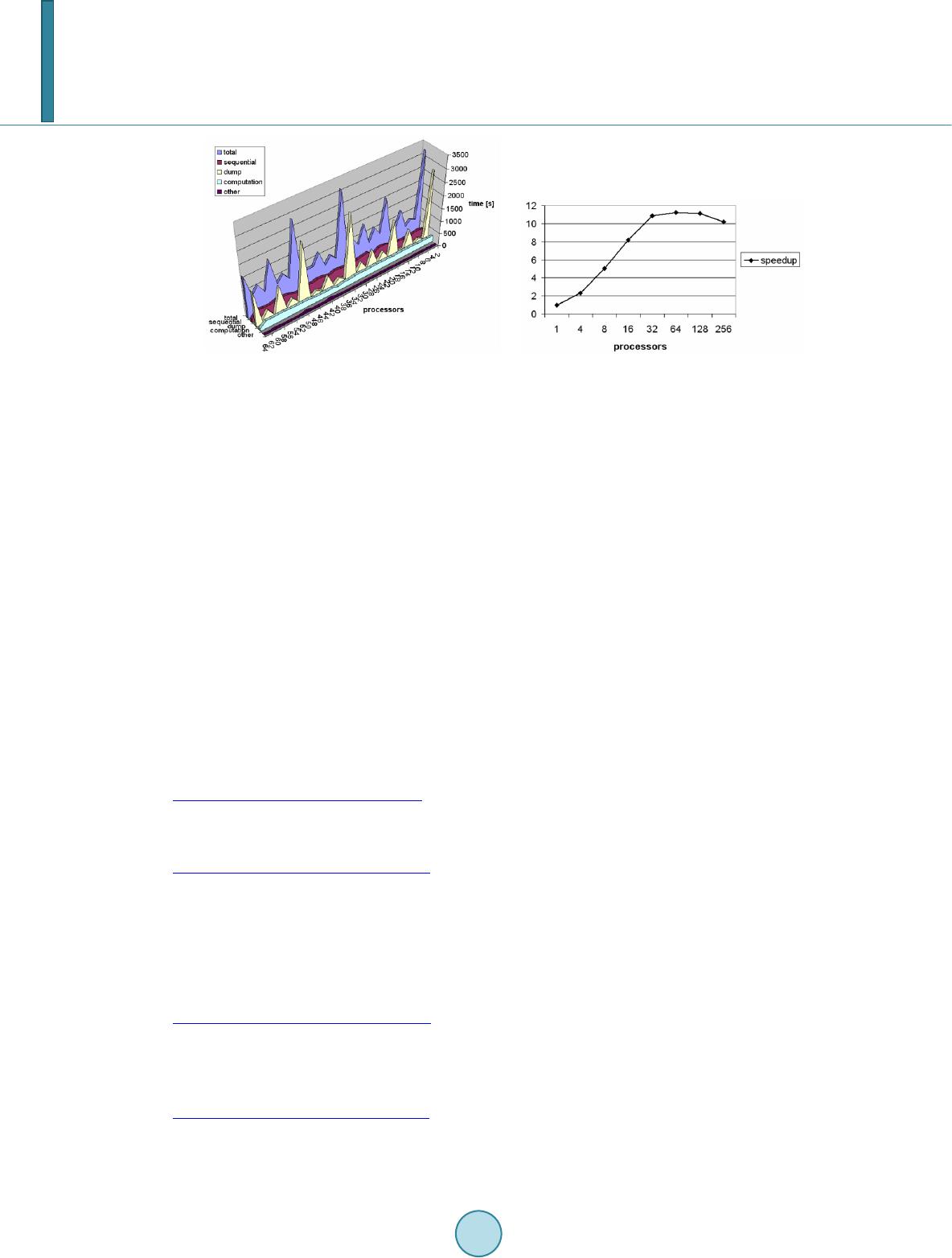

M. Sieniek et al.
1052
Figure 4. Left panel: Comparison of computations time and dump out/dump in times. Right panel: The
efficiency of the solver is limited by the efficiency of the parallel file system.
6. Conclusions
• We presented the parallel algorithm for the out-of-core multi-frontal direct solver dedicated to multi-physics
simulations.
• The advantage of our algorithm is that it allows to reduce the memory usage by dumping out all the frontal
matrices to the disc.
• The communication in the parallel algorithm occurs through a parallel data storage system.
• The parallel solver scales up to 32 processors, and its scalability is connected with the performance of the
parallel file system.
• The solver allowed for efficient solution of the challenging problem of acoustics of the human head.
Acknowledgements
The work of MP presented in this paper has been supported by Polish National Science Center grants no.
2012/06/M/ST1/00363 and 2011/01/B/ST6/00674. The work of PG and MS presented in this paper has been
supported by Polish National Science Center grant no. 2011/03/N/ST6/01397.
References
[1] Sien iek, M. and Paszyński, M. (2014) Subtree Reuse in Mult i -Frontal Solvers for Regular Grids in Step-and-Flash Im-
print Nanolithography Modeling. Advanced Engineering Materials, 16, 231-240.
http://dx.doi.org/10.1002/adem.201300267
[2] Demko wicz, L., Gatto, P., Kurtz, J., P aszynski, M., Rachowicz, W., B leszynski, E., Bleszynski, M., Hamilton, M. and
Champlin, C. (2010) Modeling of Bone Conduction of Sound in the Human Head Using hp Finite Elements I. Code
Design and Verification. Computer Methods in Applied Mechanics and Engineering, 200, 1757-1773.
http://dx.doi.org/10.1016/j.cma.2011.02.001
[3] P aszyński, M. (2013 ) Minimizing the Memory Usage with Parallel Out-of-Core Multi-Frontal Direct Solver. Computer
Assisted Mechanics and Engineering Sciences, 20, 15-41.
[4] Demko wicz, L., Kur tz, J., Par do, D., Paszyński, M., Rachowicz, W. and Zdunek, A. (2007) Computing with hp-Ada-
ptive Finite Elements, vol. II. Three Dimensional Elliptic and Maxwell Problems with Applications. Chapmann & Hall,
CRC Press.
[5] Paszyński, M., Pardo, D., Torres-Verdin, C., Demkowicz, L. and Ca l o, V. (2010) A Parallel Direct Solver for the Self-
Adaptive hp Finite Element Method. Journal of Parallel and Distributed Computing, 70, 270-281.
http://dx.doi.org/10.1016/j.jpdc.2009.09.007
[6] P aszyński, M. and Sch aefer, R. (2010) Graph Grammar Driven Parallel Partial Differential Equation Solver. Concur-
rency & Computations, Practise & Experience, 22, 1063-1097 .
[7] P aszyński, M., Pard o, D. and P aszyńska, A. (2010) Parallel Multi-Frontal Solver for p Adaptive Finite Element Mod-
eling of Multi-Physics Computational Problems. Journal of Computational Science, 1, 48-54.
http://dx.doi.org/10.1016/j.jocs.2010.03.002