Paper Menu >>
Journal Menu >>
 Theoretical Economics Letters, 2011, 1, 3-7 doi:10.4236/tel.2011.11002 Published Online May 2011 (http://www.SciRP.org/journal/tel) Copyright © 2011 SciRes. TEL The Dynamics of Wealth Inequality under Endogenous Fertility: A Remark on the Barro-Becker Model with Heterogenous Endowments Stefano Bosi1, Raouf Boucekkine2,3, Thomas Seegmuller4 1THEMA and Universit y of C e rgy- P o nt oi se , Cergy, France 2IRES and CORE, Catholic University of Louvain, Louvai n -La -Neuve, Belgium 3GREQAM, Aix-Marseille University, Marseille, France 4CNRS and GREQAM, Paris, France E-mail: stefano.bosi@u-cergy.fr, {raouf.boucekkine, thomas.seegmuller}@univmed.fr Received April 13, 2011; revised April 24, 2011; accepted April 27, 2011 Abstract Implicit in the seminal contribution of Barro-Becker [1], the lack of persistence of inequality in the pre- sence of endogenous fertility is one of the most striking features of the models à la Barro-Becker. In this pedagogical note, we show how to uncover and interpret the latter property using standard optimization in contrast to the dynamic programming under homogeneity usually invoked in this literature. Keywords: Endogenous Fertility, Heterogeneous Households, Optimal Growth 1. Introduction Following the paper by Chatterjee [2], several contri- butions hav e introduced households’ he terogeneity in the Ramsey model through wealth inequality. The main focus of this recent literature is the existence of a repre- sentative consumer summarizing the average behavior of the economy and the persistence of inequalities during the transitional dynamics and in the steady state. These questions have been extensively studied by Chatterjee, Caselli and Ventura and Garcia- Peñalosa and Turnovsky [2-4] in the standard setup where households derive utility from consumption on ly. These papers show that while wealth inequalities may be reduced, they do persist in the long-run. In contrast, another much thinner literature introducing endogenous fertility in line with Barro and Becker [1,5] has shown that inequalities do not persist. Implicit in these seminal papers, this striking property has been demonstrated in a quite general model using dynamic programming with homogenous functions by Alvarez [6]. Precisely because it is a general approach and because it does not rely on easily interpretable Euler equations, the latter framework is not reader-friendly. This note makes use of standard optimization and the resulting Euler equations to provide a simple and intui- tive reading of the lack of inequality persistence in the Barro-Becker models. More concretely, we show that when households smooth consumption over time and optimally choose the number of children, individual con- sumptions should be equal after one period. This striking property essentially derives from the resulting equality between the marginal benefit and cost of bequest: con- sumptions are then shown to be independent of the ca- pital distribution after one period. This in turn implies that fertility rates and capital held by each household become also identical after one period. Therefore, intro- ducing endogenous fertility in the optimal growth model rules out wealth inequalities after only one adjustment period. Finally, it is important to no tice that we show our result for a given sequence of prices over time. This means that it does not depend on the specification of the production sector, and occurs under exogenous as well as endogenous growth. This note is organized as follows. In the next section, we present the behavior of heterogeneous households. In Section 3, we show our result on the loss of hetero- geneity after one period, while some technical details are reported in the Appendix. 2. Households’ Behavior We extend the Barro and Becker model [5] to account for wealth heterogeneity. We consider an eco- nomy with H dynasties of altruistic households, =1,,iH, that  S. BOSI ET AL. Copyright © 2011 SciRes. TEL 4 differ in their individual wealth. In other words, we focus on heterogeneity in initial capital endowment 0i k, i.e. 00hj kk for hj. As in the seminal setting, each person is assumed to live for two periods, childhood and adulthood, and has children at the beginning of his adult period. Parents are altruistic towards their children, i.e. utility depends on their own consumption, the nu mber of surviving children and the utility of each child. The utility of an adult of type i belonging to the generation born at 1t , is given by: 1 = itititit it Uuc nnU (1) where it c is the individual consumption giving an instantaneous utility it uc , while it n is the number of children. We notice that it n measures the degree of altruism towards each child, with ,0,1 , and 1it U is the utility attained by each child. We further assume: Assumption 1 The utility function i uc is defined on R, two-times continuously differentiable on R , strictly increasing ( >0 i uc ), strictly concave ( <0 i uc ) and satisfies 2>1 ii i ucuc uc .1Noting = iiii ccucuc , we assume 0< <1 i c and i c is non-increasing. Notice that the utility function = ii uc c , with <1 , satisfies As sum ption 1.2 As stressed by Becker and Barro [1], the recursive model (1) can be equivalently written as an optimal growth model where the household of type i maximizes a dynastic utility: 1 =0 tit it t Nuc (2) with it N the size of the ith subpopulation at period t, under a sequence of budget constraints: 1=1 itit itt ittit cnkRkwn (3) =0,1,t, and given the unequal distribution of initial capital 0i k, with 00hj kk for hj. The left-hand side of (3) represents households’ ex- penditures. In particular, 1it k represents the bequest per child, through physical as well as human capital used for production in the next period. The right-hand side of (3) represents the disposable income, where t w is the wage rate and 1 tt Rr the gross return on capital, with 0,1 the depreciation rate of capital and t r the real interest rate. As mentioned in the introduction, we do not specify the production sector in order to highlight that our result holds irrespective of the production technology. Accordingly, we assume that the sequence of prices , tt wR , =0,1,t, is given. At adulthood, each household is endowed with one unit of time that she shares between labor and leisure. The time cost of rearing children is given by it t nw , where is the constant cost per child in units of time. Leisure time =1 0,1 it it nl is spent with children, whereas it l is the individual labor supply at period t. Since it n represents the population growth factor of dynasty i, the size of a dynasty at time t is given by: 1 11 0 =0 == t itit itiis s NnNNn (4) where 0>0 i N are given for =1,,iH, and hete- rogeneous initial population sizes are not excluded, i.e. 00hj NN for hj . Maximizing utility (2) under the budget constraints (3), the household i chooses a sequence 1=0 ,, ititit t knc of saving, consumption, number of children. The house- hold behavior m a y be summarized by:3 1 1= t ittititit it Rkwncnk (5) 11 = ititit t uc ucnR (6) 11 1=1 1 = ts itittitisis st it Nuc wkNuc n (7) with the transversality condition: 11=0 lim titititit tNucnk Equation (5) is the household's budget constraint. The intertemporal trade-offs are summarized by (6) and (7). The Euler Equation (6) shows how dynasties smooth consumption over time. Since the marginal utility of consumption depends on population size it N and total bequest 1it it nk , which in turn depend on the number of children, this choice between current and future con- sumption depends on the fertility rate. Finally, Equation (7) determines the optimal number of children. The cost per child in unit of time and in terms of bequest (on the left-hand side) is equal to the discounted sum of the marginal utility gains over all the subsequent periods (on the right-hand side). 3. The “Loss” of Heterogeneity Using the optimal behavior of the households, we show now that from period 1 onwards, the individual consum- ptions it c, the number of children it n and the wealth 1As it is explicitly shown in Becker and Barro [7], this inequality en- sures that the second order conditions are satisfied for the house- holds’ utility maximization. 2This utility function is considered in the seminal contribution of an d Barro and Becker [5]. 3See the Appendix for details.  S. BOSI ET AL. Copyright © 2011 SciRes. TEL 5 it k become equal. As underlined above, this property is demonstrated without specifying the production sector, the sequence of prices , tt wR , for =0,1,t, is given. As explained in the Appendix, Equation (7) can also be written as: 111111 1 1 = ititt ittit itittit ucu cRkwc nu cwk (8) Substituting Equation (6), we get: 1 111 1 1=, for =0,1,, and =1,, it itt tt it c cwRw c tiH (9) Under Assumption 1, there is a unique solution 1it c solving this equation. In other words, for all =1,t and =1, ,iH, we have it t cc , with 1 =1 t tttt t c cwRw c (10) From period =1t onwards, the individual consump- tions are equal. One can see that t c is increasing in the time cost per child measured in physical units of the next period, because the dynasty substitutes investment in children for future consumption. However, less children means a lower labor force, which explains that con- sumption is decreasing in the current wage. Most importantly for our purpose, individual consum- ptions get equalized because it c does not depend on capital holding it k and, therefore, it is independent of the distribution of capital. Indeed, recall that 1it k represents the bequest per child given by a parent living at period t. Equation (8), represents the intertemporal trade-off to have children: it equalizes the marginal benefit to have children (on the left-hand side) to its marginal cost (on the right-hand side). In particular, 111itt it uc Rk represents the marginal benefit of bequest, while 1itit it nu ck is its marginal cost. Tak- ing into account the optimal choice between current and future consumption (see (6)), the marginal benefit of bequest becomes equal to its marginal cost, implying individual consumption to be independe nt of wealth. Since consumptions are identical from =1t, the Eu- ler Equation (6) implies that the fertility rates are also identical from =1t, i.e. it t nn for all =1,t and =1,,iH. Using (10), we obtain: 11 = ttt t nR ucuc (11) Because consumptions do not depend on the wealth distribution and get equalized across dynasties, the number of child is also equalized for =1,t. A question now emerges. What can we infer for in- dividual wealth? We show that capital distribution be- comes also homogenous from period =1t. Proposition 1 Under Assumption 1, for =1,t, the distribution of capital is also homogeneous, i.e. = it t kk for all =1, ,iH. Proof. Using (5) and (7), we get: 1 =1 1 =st is tit ittis st it it N Rkcwu c uc N (12) We have = it t cc and = it t nn for all =1,t, and 1 1=1 =s is it t NN n . Therefore, Equation (12) writes for =1t: 1 1 1 111 1=2 =1 1 1 =s s its st Rkwcnuc uc (13) This shows that the capital distribution is homo- geneous at =1t, i.e. 11i kk for all =1,,iH . From =1t, the budget constraint (5) becomes: 1 1 =ttt t it it tt wnc R kk nn (14) Since 111 == ij kkk for all ,=1, ,ij H, we deduce that = itjt t kkk for all ,=1, ,ij H and =1,t This proves that the capital distribution is equal from =1t onwards. This proposition shows that introducing endogenous fertility in the optimal growth model with heterogeneous households has critical implications for the capital dis- tribution. In contrast to previous contributions with exo- genous population size starting with Chatterjee [2], ineq- uality does not persist and the wealth distribution beco- mes homogenous from =1t. As already emphasized, this arises from the disjunction between individual con- sumptions and capital holdings, which is explained by the fact that households do not only make an inter- temporal choice between present and future consump- tions, but also optimally choose the number of their children. We now come to some observations on the robu stness of our findings. Remark 1. In our analysis, we assume that the counterpart of having children is a time cost per child t w . Another traditional cost specification is to consider a cost in terms of the final good, i.e. t w [1,5]. One may easily see that this alternative specification of the cost per child does not change our conclusions on the loss of heterogeneity from =1t. Remark 2. As already underlined, our result is shown for a given sequence of prices , tt wR , =0, ,t This means that it neither depends on the microeconomic  S. BOSI ET AL. Copyright © 2011 SciRes. TEL 6 foundations of the production sector, nor on the assumptions on the technology. As a direct implication, if one introduces a standard convex technology with constant returns, the economy may obviously converge to a steady state with a homogenous wealth distribution. If one introduces a technology leading to endogenous growth [8], there may exist a unique balanced growth path where all the individuals have the same wealth growing at a similar well-defined rate. 4. References [1] F. Alvarez, “Social Mobility: The Barro-Becker Children Meet the Laitner-Loury Dynasties,” Review of Economic Dynamics, Vol. 2, No. 1, 1999, pp. 65-103. doi:10.1006/redy.1998.0052 [2] R. J. Barro and G. S. Becker, “Fertility Choice in a Model of Economic Growth,” Econometrica, Vol. 57, No. 2, 1989, pp. 481-501. doi:10.2307/1912563 [3] G. S. Becker and R. J. Barro, “A Reformulation of the Economic Theory of Fertility,” Quarterly Journal of Eco- nomics, Vol. 103, No. 1, 1988, pp. 1-25. doi:10.2307/1882640 [4] G. S. Becker and R. J. Barro “A Reformulation of the Economic Theory of Fertility,” The Quarterly Journal of Economics, Vol. 103, No. 1, 1988, pp. 1-25. doi:10.2307/1882640 [5] S. Bosi and T. Seegmuller, “Mortality Differential and Growth: What Do We Learn from the Barro-Becker Mo- del?” Mathematical Population Studies, Forthcoming , 2010 . [6] F. Caselli and J. Ventura, “A Representative Consumer Theory of Distribution,” American Economic Review, Vol. 90, No. 4, 2000, pp. 909-926. doi:10.1257/aer.90.4.909 [7] S. Chatterjee, “Transitional Dynamics and the Distribu- tion of Wealth in a Neoclassical Growth Model,” Journal of Public Economics, Vol. 54, No. 1, 1994, pp. 97-119. doi:10.1016/0047-2727(94)90072-8 [8] C. Garcia-Peñalosa and S. J. Turnovsky, “The Dynamics of Wealth Inequality in a Simple Ramsey Model: A Note on the Role of Production Flexibility,” Macroeconomic Dynamics, Vol. 13, No. 2, 2009, pp. 250-262. doi:10.1017/S1365100508070508 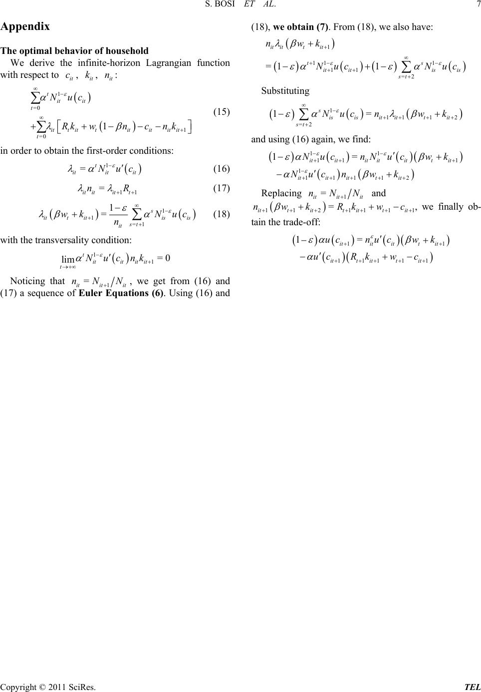 S. BOSI ET AL. Copyright © 2011 SciRes. TEL 7 Appendix The optimal behavior of household We derive the infinite-horizon Lagrangian function with respect to it c, it k, it n: 1 =0 1 =0 1 tit it t itt ittitititit t Nuc Rkwncn k (15) in order to obtain the first-order conditions: 1 =t itit it Nuc (16) 11 = it ititt nR (17) 1 1=1 1 =s ittitisis st it wk Nuc n (18) with the transversality condition: 11=0 lim titititit tNucnk Noticing that 1 = it it it nNN , we get from (16) and (17) a sequence of Euler Equations (6). Using (16) and (18), we obtain (7). From (18), we also have: 1 11 1 11 =2 =1 1 it ittit ts ititis is st nwk Nuc Nuc Substituting 11112 =2 1= sisisit ittit st Nucnw k and using (16) again, we find: 11 11 1 1111 12 1= ititit itittit itit ittit NucnNuc wk Nuc nwk Replacing 1 = it it it nNN and 112 1111 = ittitt ittit nwk Rkwc , we finally ob- tain the trade-off: 11 11111 1= ititittit ittittit ucnucwk ucRkwc |

