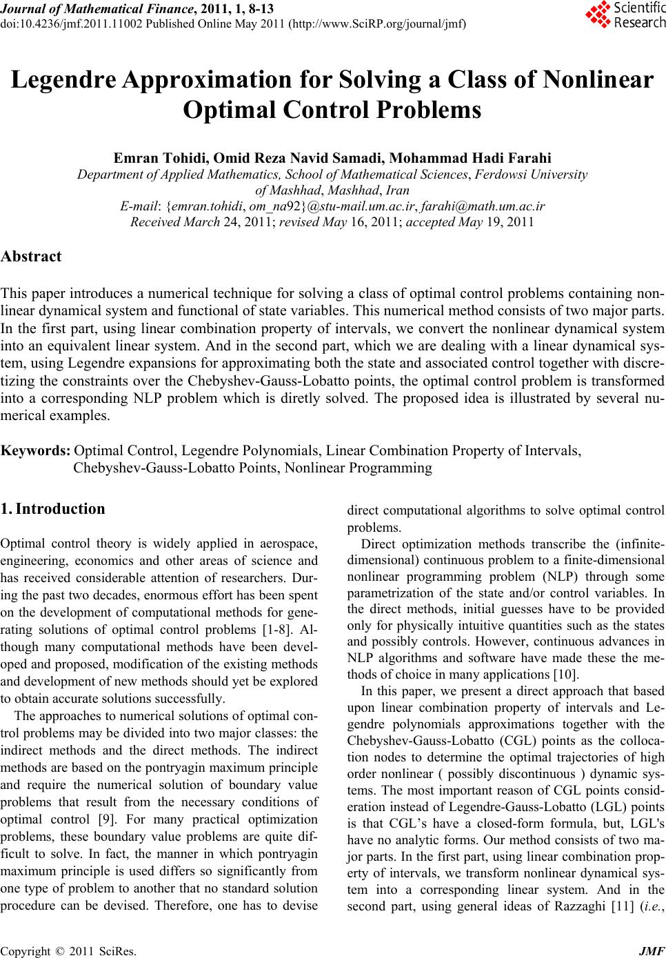Journal of Mathematical Finance, 2011, 1, 8-13
doi:10.4236/jmf.2011.11002 Published Online May 2011 (http://www.SciRP.org/journal/jmf)
Legendre App roximation for Solving a Class of Nonlinear
Optimal Control Problems
Emran Tohidi, Omid Reza Navid Samadi, Mohammad Hadi Farahi
Department of Applied Mathematics, School of Mathematical Sciences, Ferdowsi University
of Mashhad, Mashhad, Iran
Received March 24, 2011; revised May 16, 2011; accepted M ay 19, 2011
Abstract
This paper introduces a numerical technique for solving a class of optimal control problems containing non-
linear dynamical system and functional of state variables. This numerical method consists of two major parts.
In the first part, using linear combination property of intervals, we convert the nonlinear dynamical system
into an equivalent linear system. And in the second part, which we are dealing with a linear dynamical sys-
tem, using Legendre expansions for approximating both the state and associated control together with discre-
tizing the constraints over the Chebyshev-Gauss-Lobatto points, the optimal control problem is transformed
into a corresponding NLP problem which is diretly solved. The proposed idea is illustrated by several nu-
merical examples.
Keywords: Optimal Control, Legendre Polynomials, Linear Combination Property of Intervals,
Chebyshev-Gauss-Lobatto Points, Nonlinear Programming
1. Introduction
Optimal control theory is widely applied in aerospace,
engineering, economics and other areas of science and
has received considerable attention of researchers. Dur-
ing the past two decades, enormous effort has been spent
on the development of computational methods for gene-
rating solutions of optimal control problems [1-8]. Al-
though many computational methods have been devel-
oped and proposed, modification of the existing methods
and development of new methods should yet be explored
to obtain accurate solutions successfully.
The approaches to numerical solutions of optimal con-
trol problems may be divided into two major classes: the
indirect methods and the direct methods. The indirect
methods are based on the pontryagin maximum principle
and require the numerical solution of boundary value
problems that result from the necessary conditions of
optimal control [9]. For many practical optimization
problems, these boundary value problems are quite dif-
ficult to solve. In fact, the manner in which pontryagin
maximum principle is used differs so significantly from
one type of problem to another that no standard solution
procedure can be devised. Therefore, one has to devise
direct computational algorithms to solve optimal control
problems.
Direct optimization methods transcribe the (infinite-
dimensional) continuous problem to a finite-dimensional
nonlinear programming problem (NLP) through some
parametrization of the state and/or control variables. In
the direct methods, initial guesses have to be provided
only for physically intuitive quantities such as the states
and possibly controls. However, continuous advances in
NLP algorithms and software have made these the me-
thods of choice in many applications [10].
In this paper, we present a direct approach that based
upon linear combination property of intervals and Le-
gendre polynomials approximations together with the
Chebyshev-Gauss-Lobatto (CGL) points as the colloca-
tion nodes to determine the optimal trajectories of high
order nonlinear ( possibly discontinuous ) dynamic sys-
tems. The most important reason of CGL points consid-
eration instead of Legendre-Gauss-Lobatto (LGL) points
is that CGL’s have a closed-form formula, but, LGL's
have no analytic forms. Our method consists of two ma-
jor parts. In the first part, using linear combination prop-
erty of intervals, we transform nonlinear dynamical sys-
tem into a corresponding linear system. And in the
second part, using general ideas of Razzaghi [11] (i.e.,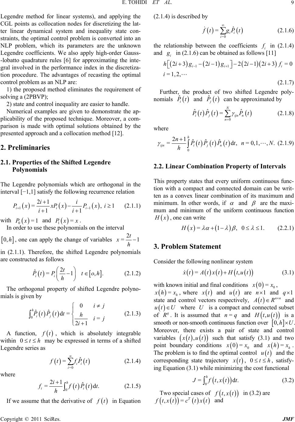

E. TOHIDI ET AL. 9
Legendre method for linear systems), and applying the
CGL points as collocation nodes for discretizing the lat-
ter linear dynamical system and inequality state con-
straints, the optimal control problem is converted into an
NLP problem, which its parameters are the unknown
Legendre coefficients. We also apply high-order Gauss-
-lobatto quadrature rules [6] for approximating the inte-
gral involved in the performance index in the discretiza-
tion procedure. The advantages of recasting the optimal
control problem as an NLP are:
1) the proposed method eliminates the requirement of
solving a (2PBVP);
2) state and control inequality are easier to handle.
Numerical examples are given to demonstrate the ap-
plicability of the proposed technique. Moreover, a com-
parison is made with optimal solutions obtained by the
presented approach and a collocation method [12].
2. Preliminaries
2.1. Properties of the Shifted Legendre
Polynomials
The Legendre polynomials which are orthogonal in the
interval [−1,1] satisfy the following recurrence relation
  
11
21
=, 1
11
iii
ii
PxxPx Pxi
ii


 (2.1.1)
with

0=1Px and

1=Px x
.
In order to use these polynomials on the interval


0, h, one can apply the change of variables 2 =1
t
xh

in (2.1.1). Therefore, the shifted Legendre polynomials
are constructed as follows
 
2
ˆ=1 ,.
ii
t
PtPt oh
h



 (2.1.2)
The orthogonal property of shifted Legendre polyno-
mials is given by
 
0
0
ˆˆd= =
21
h
ij
ij
PtPt thij
i






 (2.1.3)
A function,

f
t, which is absolutely integrable
within 0th may be expressed in terms of a shifted
Legendre series as
 
=0
ˆ
=ii
i
f
tfPt

 (2.1.4)
where
 
0
21 ˆ
=d.
h
ii
i
f
ftPt t
h
 (2.1.5)
If we assume that the derivative of


f
t in Equation
(2.1.4) is described by
 
=0
ˆ
=ii
i
f
tgPt


 (2.1.6)
the relationship between the coefficients i
f
in (2.1.4)
and i
g
in (2.1.6) can be obtained as follows [11]




11
232122123 =0
=1,2,
ii i
higi giif
i

 


(2.1.7)
Further, the product of two shifted Legendre poly-
nomials


ˆi
Pt and


ˆj
Pt can be approximated by
 
0
ˆˆ ˆ
=
N
ijijn n
n
PtPt Pt 

 (2.1.8)
where
 
0
21
ˆˆ ˆ
=d, =0,1,,.
h
ijnij n
nPtPtPtt nN
h

(2.1.9)
2.2. Linear Combination Property of Intervals
This property states that every uniform continuous func-
tion with a compact and connected domain can be writ-
ten as a convex linear combination of its maximum and
minimum. In other words, if

and

are the maxi-
mum and minimum of the uniform continuous function


H
x, one can write




=1, 01.Hx  

 (2.2.1)
3. Problem Statement
Consider the following nonlinear system





 
=,
x
tAtxtHtut
 (3.1)
with known initial and final conditions

0
0=
x
x,


=h
x
hx , where


x
t and

ut are 1n and 1q

state and control vectors respectively,

nn
A
tR

 and


ut U

where U is a compact and connected subset
of q R. It is assumed that =nq and

 
,
H
tut is a
smooth or non-smooth continuous function over


0, hU

.
Moreover, there exists a pair of state and control
variables






,
x
tut such that satisfy (3.1) and two
point boundary conditions

0
0=
x
x and


=h
x
hx.
The problem is to find the optimal control

ut and the
corresponding state trajectory

x
t, 0th , satisfy-
ing Equation (3.1) while minimizing the cost functional
 
0
=,d.
h
J
ftxt t
 (3.2)
Two special cases of



,
f
txt in (3.2) are








,=
T
f
txtctxt and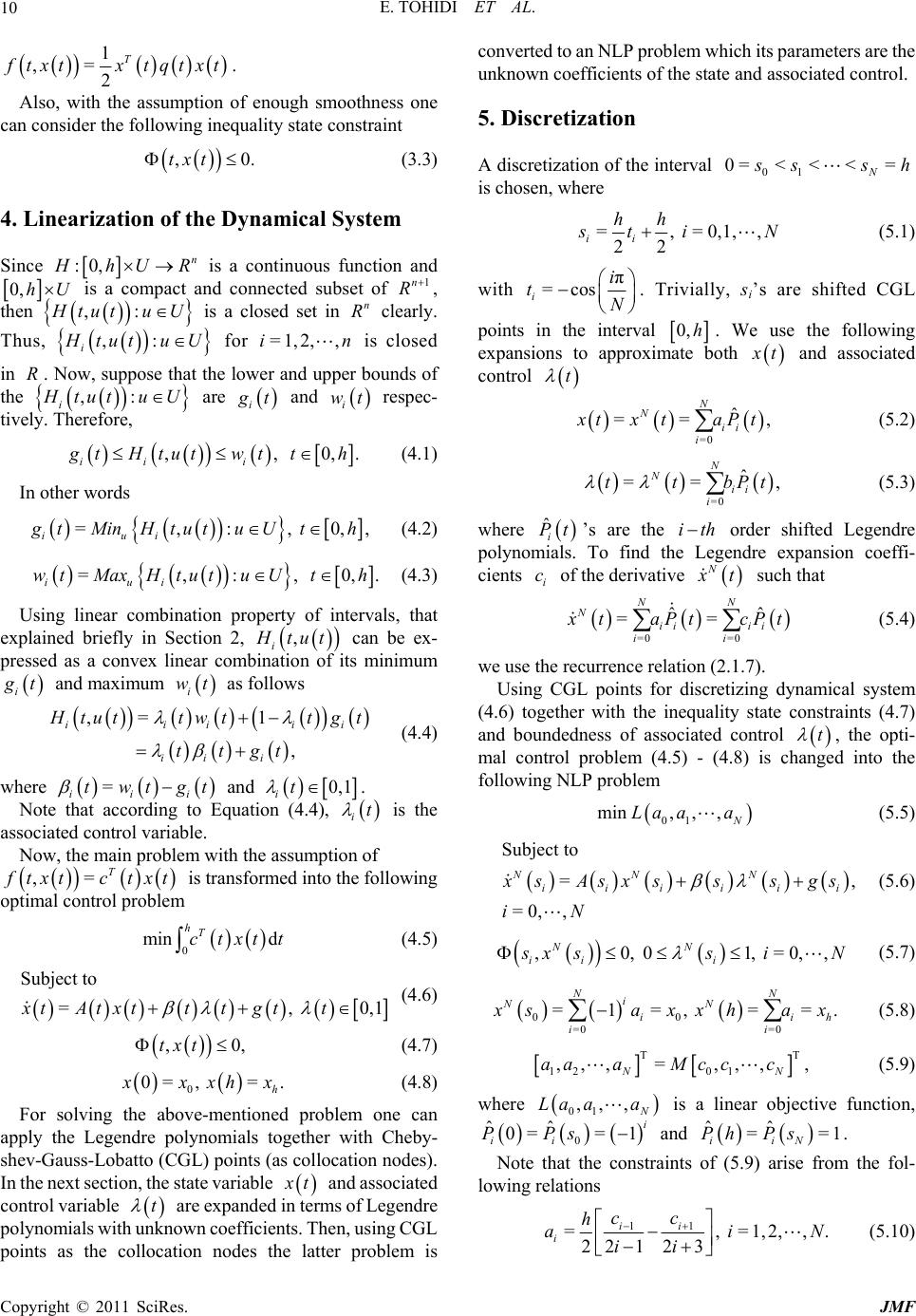

E. TOHIDI ET AL. 10
    
1
,=
2
T
f
txtxtqtxt .
Also, with the assumption of enough smoothness one
can consider the following inequality state constraint
 
,0.txt (3.3)
4. Linearization o f th e Dy na mi ca l S ys te m
Since


:0, n
H
hU R is a continuous function and


0, hU is a compact and connected subset of 1n
R

,
then
 

,:
H
tutu U is a closed set in n R clearly.
Thus,
 

,:
i
H
tutu U for =1,2, ,in is closed
in R. Now, suppose that the lower and upper bounds of
the
 

,:
i
H
tutu U are

i
g
t and

i
wt respec-
tively. Therefore,
    

,, 0,.
ii i
g
tHtut wtth (4.1)
In other words
  


=,:, 0,,
iui
g
tMinHtutuUth (4.2)
  


=,:, 0,.
iui
wtMaxHtutu Uth (4.3)
Using linear combination property of intervals, that
explained briefly in Section 2,
 
,
i
H
tut can be ex-
pressed as a convex linear combination of its minimum

i
g
t and maximum

i
wt as follows
     
 
,= 1
,
iiiii
ii i
H
tutt wttgt
ttgt



 (4.4)
where
 
=
iii
twtgt   and
 

0,1
it
 .
Note that according to Equation (4.4),

it
 is the
associated control variable.
Now, the main problem with the assumption of
   
,=
T
f
txtctxt is transformed into the following
optimal control problem

0
min d
hT
ctxtt
 (4.5)
 
Subject to
=, 0,1xtAtxttt gtt    
 (4.6)



,0,txt (4.7)
 
0
0=, =.
h
x
xxh x (4.8)
For solving the above-mentioned problem one can
apply the Legendre polynomials together with Cheby-
shev-Gauss-Lobatto (CGL) points (as collocation nodes).
In the next section, the state variable

x
t and associated
control variable

t  are expanded in terms of Legendre
polynomials with unknown coefficients. Then, using CGL
points as the collocation nodes the latter problem is
converted to an NLP problem which its parameters are the
unknown coefficients of the state and associated control.
5. Discretization
A discretization of the interval 01 0=< <<=
N
s
ssh
is chosen, where
=, =0,1,,
22
ii
hh
s
ti N (5.1)
with π =cos
ii
tN



. Trivially, si’s are shifted CGL
points in the interval


0, h. We use the following
expansions to approximate both


x
t and associated
control


t 
 
=0
ˆ
== ,
N
Nii
i
x
txt aPt
 (5.2)
 
=0
ˆ
== ,
N
Nii
i
ttbPt 
 (5.3)
where


ˆi
Pt’s are the ith

order shifted Legendre
polynomials. To find the Legendre expansion coeffi-
cients i c of the derivative

N
x
t
 such that
 
=0 =0
ˆˆ
==
NN
Nii ii
ii
x
taPtcPt


 (5.4)
we use the recurrence relation (2.1.7).
Using CGL points for discretizing dynamical system
(4.6) together with the inequality state constraints (4.7)
and boundedness of associated control

t  , the opti-
mal control problem (4.5) - (4.8) is changed into the
following NLP problem


01
min ,,,
N
La aa (5.5)
 
Subject to
=,
=0,,
NNN
iiiiii
x
sAsxss sgs
iN
 


(5.6)





,0, 01, =0,,
NN
ii i
s
xss iN   (5.7)
  
00
=0 =0
=1=, ==.
NN
i
NN
iih
ii
x
saxxhax

(5.8)

TT
12 01
,,,=,,, ,
NN
aaaMcc c
(5.9)
where


01
,,,
N
La aa is a linear objective function,



0
ˆˆ
0== 1
i
ii
PPs

and


ˆˆ
==1
iiN
Ph Ps.
Note that the constraints of (5.9) arise from the fol-
lowing relations
11
=, =1,2,,.
221 23
ii
i
cc
h
aiN
ii






 (5.10)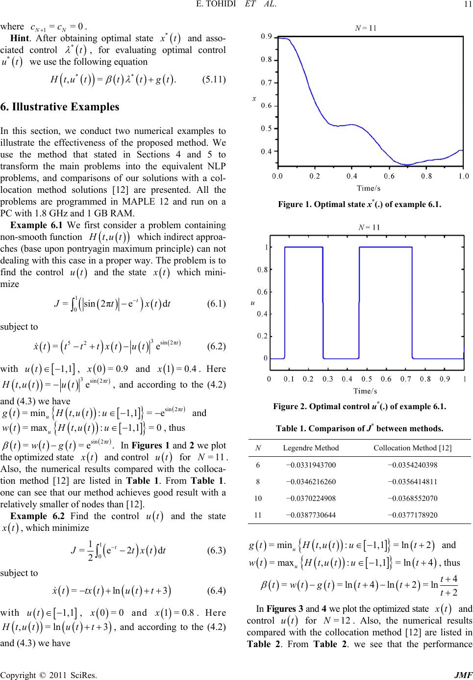

E. TOHIDI ET AL. 11
where 1==0
NN
cc
.
Hint. After obtaining optimal state

*
x
t and asso-
ciated control

*t
 , for evaluating optimal control

*
ut we use the following equation


 
**
,= .
H
tu tttgt   (5.11)
6. Illustrative Examples
In this section, we conduct two numerical examples to
illustrate the effectiveness of the proposed method. We
use the method that stated in Sections 4 and 5 to
transform the main problems into the equivalent NLP
problems, and comparisons of our solutions with a col-
location method solutions [12] are presented. All the
problems are programmed in MAPLE 12 and run on a
PC with 1.8 GHz and 1 GB RAM.
Example 6.1 We first consider a problem containing
non-smooth function


,
H
tut which indirect approa-
ches (base upon pontryagin maximum principle) can not
dealing with this case in a proper way. The problem is to
find the control

ut and the state

x
t which mini-
mize



1
0
=sin2πed
t
J
txtt


 (6.1)
subject to


 

3sin 2π
52
=e
t
xtt ttxtut 
 (6.2)
with
 

1,1ut ,

0=0.9x and

1=0.4x. Here




3sin 2π
,= e
t
Htut ut, and according to the (4.2)
and (4.3) we have
   


sin 2π
=min,:1,1 = et
u
gtHtut u and
   

=max,:1,1 =0
u
wtHtut u , thus


sin 2π
==e.
t
twtgt   In Figures 1 and 2 we plot
the optimized state

x
t and control

ut for =11N.
Also, the numerical results compared with the colloca-
tion method [12] are listed in Table 1. From Table 1.
one can see that our method achieves good result with a
relatively smaller of nodes than [12].
Example 6.2 Find the control

ut and the state

x
t, which minimize


1
0
1
=e2 d
2
t
J
txt t

 (6.3)
subject to
 


=ln 3xttxtut t 
 (6.4)
with
 

1,1ut ,

0=0x and

1=0.8x. Here




,=ln 3Htutut t , and according to the (4.2)
and (4.3) we have
Figure 1. Optimal state x*(.) of example 6.1.
Figure 2. Optimal control u*(.) of example 6.1.
Table 1. Comparison of J* between methods.
NLegendre Method Collocation Method [12]
6−0.0331943700 −0.0354240398
8−0.0346216260 −0.0356414811
10 −0.0370224908 −0.0368552070
11 −0.0387730644 −0.0377178920
 






=min,:1,1 =ln2
u
gtHtut ut

 and
 

 



=max,:1,1 =ln4
u
wtHtut ut , thus

4
==ln4ln2=ln
2
t
twtgt ttt




In Figures 3 and 4 we plot the optimized state


x
t and
control


ut for =12N. Also, the numerical results
compared with the collocation method [12] are listed in
Table 2. From Table 2. we see that the performance

E. TOHIDI ET AL. 12
Figure 3. Optimal state x*(.) of example 6.2.
Figure 4. Optimal control u*(.) of example 6.2.
Table 2. Comparison of J* between methods.
N Legendre Method Collocation Method [12]
7 −0.1820295698 −0.1815318828
9 −0.1825806940 −0.1821287778
11 −0.1826754624 −0.1823052407
12 −0.1828354838 −0.1826714837
index got by our approach are better than those obtained
by the method in [12].
7. Conclusions
The aim of the present work is the determination of the
optimal control and state vectors by a direct method of
solution based upon linear combination property of in-
tervals and shifted Legendre series expansions together
with the CGL points as collocation nodes respectively.
The method is based upon reducing a nonlinear optimal
control problem to an NLP. The unity of the weight
function of orthogonality for shifted Legendre series and
the simplicity of the discretization are merits that make
the approach very attractive. Moreover, only a small
number of shifted Legendre series is needed to obtain a
very satisfactory solution. The given numerical examples
supports this claim.
8. References
[1] R. R. Bless, D. H. Hoges and H. Seywald, “Finite Ele-
ment Method for the Solution of State-Constrained Op-
timal Control Problems,” Journal of Guidance, Control,
and Dynamics, Vol. 18, No. 5, 1995, pp. 1036-1043.
doi:10.2514/3.21502
[2] R. Bulrisch and D. Kraft, “Computational Optimal Con-
trol,” Birkhauser, Boston, 1994.
[3] G. Elnagar, M. A. Kazemi and M. Razzaghi, “The Pseu-
dospectral Legendre Method for Discretizing Optimal
Control Problems,” IEEE Transactions on Automatic C on-
trol, Vol. 40, No. 10, 1995, pp. 1793-1796.
doi:10.1109/9.467672
[4] G. N. Elnagar and M. A. Kazemi, “Pseudospectral Che-
byshev Optimal Control of Constrained Nonlinear Dy-
namical Systems,” Computational Optimization and Ap-
plications, Vol. 11, No. 2, 1998, pp. 195-217.
doi:10.1109/9.467672
[5] W. W. Hager, “Multiplier Methods for Nonlinear Optim-
al Control Problems,” SIAM Journal on Numerical Anal,
Vol. 27, No. 4, 1990, pp. 1061-1080.
doi:10.1137/0727063
[6] A. L. Herman and B. A. Conway, “Direct Trajectory
Optimization Using Collocation Based on High-Order
Gauss-Lobatoo Quadrature Rules,” Journal of Guidance,
Control, and Dynamics, and Dynamics, Vol. 19, No. 3,
1996, pp. 592-599. doi:10.2514/3.21662
[7] M. Ross and F. Fahroo, “Legendre Pseudospectral Ap-
proximations of Optimal Control Problems,” Lecture Note s
in Control and Information Sciences, Vol. 295, No. 1,
2003, pp. 327-342.
[8] J. Vlassenbroeck and R. V. Dooren, “A Chebyshev Tech-
nique for Solving Nonlinear Optimal Control Problems,”
IEEE Transactions on Automatic Control, Vol. 33, No. 4,
1988, pp. 333-340. 10.1109/9.192187
[9] H. Seywald and R. R. Kumar, “Finite Difference Scheme
for Automatic Costate Calculation,” Journal of Guidance,
Control, and Dynamics, and Dynamics, Vol. 19, No. 1,
1996, pp. 231-239. doi:10.2514/3.21603
[10] K. Schittkowskki, “NLPQL: A Fortran Subroutine for

E. TOHIDI ET AL. 13
Solving Constrained Nonlinear Programming Problems,”
Operations Research Annals, Vol. 5, No. 2, 1985, pp.
385-400.
[11] M. Razzaghi and G. Elnagar, “A Legendre Technique For
Solving Time-Varing Linear Quadratic Optimal Control
Problems,” Journal of the Franklin Institute, Vol. 330,
No. 3, 1993, pp. 453-463.
doi:10.1016/0016-0032(93)90092-9
[12] O. V. Stryk, “Numerical Solution of Optimal Control
Problems by Direct Collocation,” In: R. Bulrisch, A.
Miele, J. Stoer and K. H. Well, Eds., Optional Control of
Variations, Optimal Control Theory and Numerical Me-
thods, International Series of Numerical Mathematics,
Birkhäuser Verlag, Basel, 1993, pp. 129-143.