Journal of Mathematical Finance, 2011, 1, 1-7
doi:10.4236/jmf.2011.11001 Published Online May 2011 (http://www.SciRP.org/journal/jmf)
The Effect of Ti ck Size on Testing for Nonlinearity in
Financial Markets Data
Heather Mitchell1, Michael McKenzie2,3
1School of Economics, Finance and Marketing, Royal Melbourne Institute of Technology, Melbourne, Australia
2Faculty of Economics and Business, University of Sydney, Sydney, Australia
3Centre for Financial Analysis and Policy, Cambridge University, Cambridge, UK
Received May 6, 2011; revised May 16, 2011; accepted May 19 , 20 11
Abstract
The discrete nature of financial markets time-series data may prejudice the BDS and Close Returns test for
nonlinearity. Our estimation results suggest that a tick/volatility ratio threshold exists, beyond which the test
results are biased. Further, tick/volatility ratios that exceed these thresholds are frequently observed in finan-
cial markets data, which suggests that the results of the BDS and CR test must be interpreted with caution.
Keywords: Compass Rose, Tick/Volatility Ratio, BDS Test, Close Returns Test
1. Introduction
A body of literature has evolved which considers the
implications of discreteness for: 1) trading behaviour [1];
2) technical trading strategies [2,3]; 3) model estimation
[4,5]; and most importantly in the current context, 4)
tests of the statistical properties of financial market d ata.
For example, Gottleib and Kalay [6] find that discrete-
ness biases the second and higher order moment esti-
mates of returns data upwards. Koppl and Tuluca and
Fang [7,8] consider the impact of the compass rose on
random walk testing. Crack and Ledoit [9] discuss how
the presence of the compass rose pattern may distort the
null distribution for the Brock, Dechert and Scheinkman
(BDS) test for nonlinearity. Kramer and Runde [10] em-
pirically test this proposition and find that the null dis-
tribution of the BDS test for chaos is distorted in the
presence of discret e ness.
The purpose of this paper is to provide further evi-
dence of the impact of discreteness on tests of the prop-
erties of financial markets data. Specifically, the BDS
test of Brock, Dechert and Scheinkman [11] and the Clo s e
Returns (CR hereafter) tests of nonlinearity are consi-
dered. The results sugg est that both the CR and BDS test
are sensitive to data discreteness, although only in sam-
ple sizes of less than 500 observations for the latt er.
2. The BDS and Close Returns Test
One of the most commonly applied tests for nonlin earity
is the BDS test of Brock, Dechert and Scheinkman [11]
details of which may be found in Dechert [12]. In es-
sence, the test simply focuses on pairs of points in the
dataset. If the series is iid, then the probability of the
distance between these points being less than or equal to
some arbitrarily chosen distance, ε will be a constant.
More formally, the BDS test is a statistical test of the
null hypothesis of IID and is based on the Grassberger
and Procaccia [13] correlation integral for a given em-
bedding dimension. If the test value is significantly dif-
ferent from a standard normal distribution, it can be con-
cluded that the giv en signal is deterministic. As such, the
BDS procedure may be considered as a test for linear and
nonlinear departures from IID rather than a specific test
for chaos. It is in this latter context however, th at the test
has most commonly been applied usually in conjunction
with the estimation of entropy, Lyapunov exponents or
correlation dimensions. The BDS test belongs to the me-
tric invariant class of tests for chaotic behaviour and an
extensive literature has emerged which uses the BDS
metric to test for nonlinear behaviour in a wide range of
financial data including: 1) stock market returns [14,15],
2) exchange rates [16,17], 3) futures data [18], 4) com-
modity prices [19,20] and 5) macroeconomic data [21].
In general, the BDS test results furnished by this litera-
ture provide substantial empirical evidence of nonlinear
structure in a wide range of financial asset prices.
An alternative nonlinear testing pro cedure is the Close
Returns (CR hereafter) test details of which may be
found in Gilmore [22]. The close returns test is a topo-

H. MITCHELL ET AL.
2
logical based testing procedure which was specifically
designed to detect low dimensional chaotic behaviour. It
is a two-part test consisting of a qualitative component
which is a graphical test for the presence of chaotic be-
haviour. The second quantitative element is a test of the
null hypothesis that the data is IID against both linear
and nonlinear alternatives. The topological approach
attempts to determine how the unstable periodic orbits of
the strange attractor are intertwined. The processes of
stretching and compression are responsible for organis-
ing the strange attractor in a unique way and if one can
determine how the unstable periodic orbits are org anised,
we can identify the stretching and compressing mechan-
isms responsible for the creation of the strange attractor.
This information is robust against noise and is indepen-
dently verifiable. Once these mechanisms have been
identified, a geometric model can be constructed which
describes how to model the stretching and squeezing
mechanisms responsible for generating the original time
series. That is to say, topological tests may not only
detect the presence of chaos (the only information pro-
vided by the metric class of tests), but can also provide
information about the underlying system responsible for
the chaotic behaviour. As the topological method pre-
serves the time ordering of the data, where evidence of
chaos is found, the researcher may proceed to characte-
rise the underlying process in a quantitative way. Thus,
one is able to reconstruct the stretching and compressing
mechanisms responsible for generating the strange at-
tractor. While not enabling the researcher to identify the
underlying equation system, it does allow the rejection of
models which produce behaviour that is incompatible
with the characteristics of the strange attractor identified
by this technique. Applicatio n s of the CR test to financial
markets data may be found in Gilmore and McKenzie
[17,22-26].
3. Random Data and the BDS and Close
Returns Test
To assess the impact of discreteness of the BDS and CR
test, we must firstly benchmark the performance of these
tests against simulated data. As such, a 1,00 0 observ ation
series of random numbers is created using the Knuth [27]
psuedo-random number generator, which is assumed to
be normally distributed with a zero mean and constant
variance equal to one.1The BDS test and CR test are then
applied to these data, which are recorded to 18 decimal
places.
When estimating the BDS test, the neighbourhood size
and the embedding dimension must be specified. As a
general guide, Brock, Hsieh and LeBaron [28] suggest an
embedding dimension of between 2 and 5 and a range for
the threshold term of 0.5 to 2. In an effort to make our
results as generalisable as possible, we extent the range
of values suggested by Brock et al. [28] and estimate the
BDS test assuming an embedding dimension of 2 - 6 and
a threshold term which ranges from 0.01 to 5.2Thus, the
BDS test is applied to each 1,000 observation simulated
data series assuming each combination of embedding
dimension and threshold term. This process is repeated
1,000 times and Panel A of Table 1 presents a summary
of the proportion of rejections of the null. The nominal
size of the test is assumed to be 0.05 in all cases and the
figures in bold indicate the instances in which the pro-
portion of rejections of the null is not significantly dif-
ferent from the nominal size of the level of significance.
The performance of the CR test when applied to a
random number series may also be considered. The CR
test requires the neighbourhood and histogram size to be
specified. Both of these values are subjective and a his-
togram length of between 400 and 600 observations is
assumed. Further, the neighbourhood size is assumed to
vary over the same range as set in the BDS test results.
The estimation results are presented in Panel B of Table
1 and the figures in bold indicate the instances in which
the proportion of rejections of the nu ll is not sig n ificantly
different from the nominal size of the level of signific-
ance.
In general, the results suggest that both the BDS and
CR test are sensitive to the specification of the neigh-
urhood size. The BDS test performs best for a threshold
value of 1.00 or 1.50 whereas the CR test performs best
for a neighbourhood size of 0.01 to 0.05. Neither test
performs well for values outside of this range as the BDS
test fails to reject the null sufficiently often, whereas the
CR test almost never fails to reject the null. The choice
of embedded dimension for the BDS test, or histogram
size for the CR test, do not appear to impact on the gen-
eral tenor of the results.
4. Discrete Data and the BDS and Close
Returns Test
The extent to which discreteness imposes itself on the
movements in prices is a function of the volatility of the
data. As such, the performance of the BDS and CR test
will be considered for simulated data that exhibits dif-
2A neighbourhood size of 7.5 and 10 was also specified, however the
BDS typically failed to furnish a result and so presenting information
as to the proportion of rejections of the null is not informative.
1To ensure that the results are driven by the tick effect and not the
p
suedo-randomness of the number generator, Knuth’s [27] lagged
Fibonacci generator, L’Ecuyer’s [29] combined multiple recursive
generator and Matsumoto and Nishimura’s [30] Mersenne Twister are
all considered. All three generators produced qualitatively consisten
t
results and so, to conserve space, the discussion shall focus solely on
the Knuth results.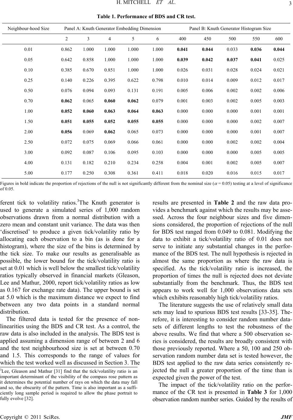

H. MITCHELL ET AL.
3
Table 1. Performance of BDS and CR test.
Neighbour-hood Size Panel A: Knuth Generator Embedding Dimen sion Panel B: Knuth Generator Histogram Size
2 3 4 5 6 400 450 500 550 600
0.01 0.862 1.000 1.000 1.000 1.000
0.041 0.044 0.033 0.036 0.044
0.05 0.642 0.858 1.000 1.000 1.000 0.039 0.042 0.037 0.041 0.025
0.10 0.385 0.670 0.851 1.000 1.000 0.026 0.031 0.028 0.024 0.021
0.25 0.140 0.226 0.395 0.622 0.798 0.010 0.014 0.009 0.012 0.017
0.50 0.076 0.094 0.093 0.131 0.191 0.005 0.006 0.002 0.002 0.006
0.70 0.062 0.065 0.060 0.062 0.079 0.001 0.003 0.002 0.005 0.003
1.00 0.052 0.060 0.063 0.064 0.063 0.000 0.000 0.000 0.001 0.001
1.50 0.051 0.055 0.052 0.055 0.055 0.000 0.000 0.000 0.002 0.007
2.00 0.056 0.069 0.062 0.065 0.073 0.000 0.000 0.000 0.001 0.007
2.50 0.072 0.075 0.069 0.066 0.061 0.000 0.000 0.002 0.002 0.004
3.00 0.092 0.087 0.106 0.095 0.103 0.000 0.000 0.000 0.005 0.005
4.00 0.131 0.182 0.210 0.234 0.258 0.004 0.001 0.002 0.005 0.007
5.00 0.177 0.250 0.308 0.361 0.411 0.018 0.020 0.016 0.015 0.017
Figures in bold indicate the proportion of rejections of the null is not significantly different from the nominal size (  = 0.05) testing at a level of significance
of 0.05.
ferent tick to volatility ratios.3The Knuth generator is
used to generate a simulated series of 1,000 random
observations drawn from a normal distribution with a
zero mean and constant unit variance. The data was then
‘discretised’ to produce a given tick/volatility ratio by
allocating each observation to a bin (as is done for a
histogram), where the size of the bins is determined by
the tick size. To make our results as generalisable as
possible, the lower bound for the tick/volatility ratio is
set at 0.01 which is well below the smallest tick/volatility
ratios typically observed in financial markets (Gleason,
Lee and Mathur, 2000, report tick/volatility ratio s as low
as 0.167 for exchange rate data). The upper bound is set
at 5.0 which is the maximum distance we expect to find
between any two data points in a standard normal
distribution.
The filtered data is tested for the presence of non-
linearities using the BDS and CR test. As a control, the
raw data is also included in the analysis. The BDS test is
applied assuming a dimension range of between 2 and 6
and the test neighbourhood size is set at between 0.70
and 1.5. This corresponds to the range of values for
which the test worked well as discussed in Section 3. The
results are presented in Table 2 and the raw data pro-
vides a benchmark against which the results may be asse-
ssed. Across the four neighbour sizes and five dimen-
sions considered, the proportion of rejections of the null
for BDS test ranged from 0.049 to 0.081. Modifying the
data to exhibit a tick/volatility ratio of 0.01 does not
serve to initiate any substantial changes in the perfor-
mance of the BDS test. The null hypothesis is rejected in
almost the same proportion as where the raw data is
specified. As the tick/volatility ratio is increased, the
proportion of times the null is rejected does not deviate
substantially from the benchmark. Thus, the BDS test
appears to work well for 1,000 observations data sets
which exhibits reasonably high tick/volatility ratios.
The literature suggests the use of relatively small data
sets may lead to spurious BDS test results [33-35]. The-
refore, it is interesting to consider random number data-
sets of different lengths to test the robustness of the
above results. We find that where a 500 observation se-
ries is considered, the results are broadly consistent with
those previously reported. Where a 50, 100 and 250 ob-
servation random number data set is tested however, the
BDS test applied to the raw data series consistently re-
jected the null a greater proportion of the time than is
expected given the power of the test.
The impact of the tick/volatility ratio on the perfor-
mance of the CR test is presented in Table 3 for 1,000
observation random number seri es. Guided b y the resu lts of
3Lee, Gleason and Mathur [31] find that the tick/volatility ratio is an
important determinant of the visibility of the compass rose pattern as
it determines the potential number of rays on which the data may fall
and so, the obscurity of the pattern. Time is also important as a suffi-
ciently long sample period is required to allow the phase portrait to
fully evolve [32].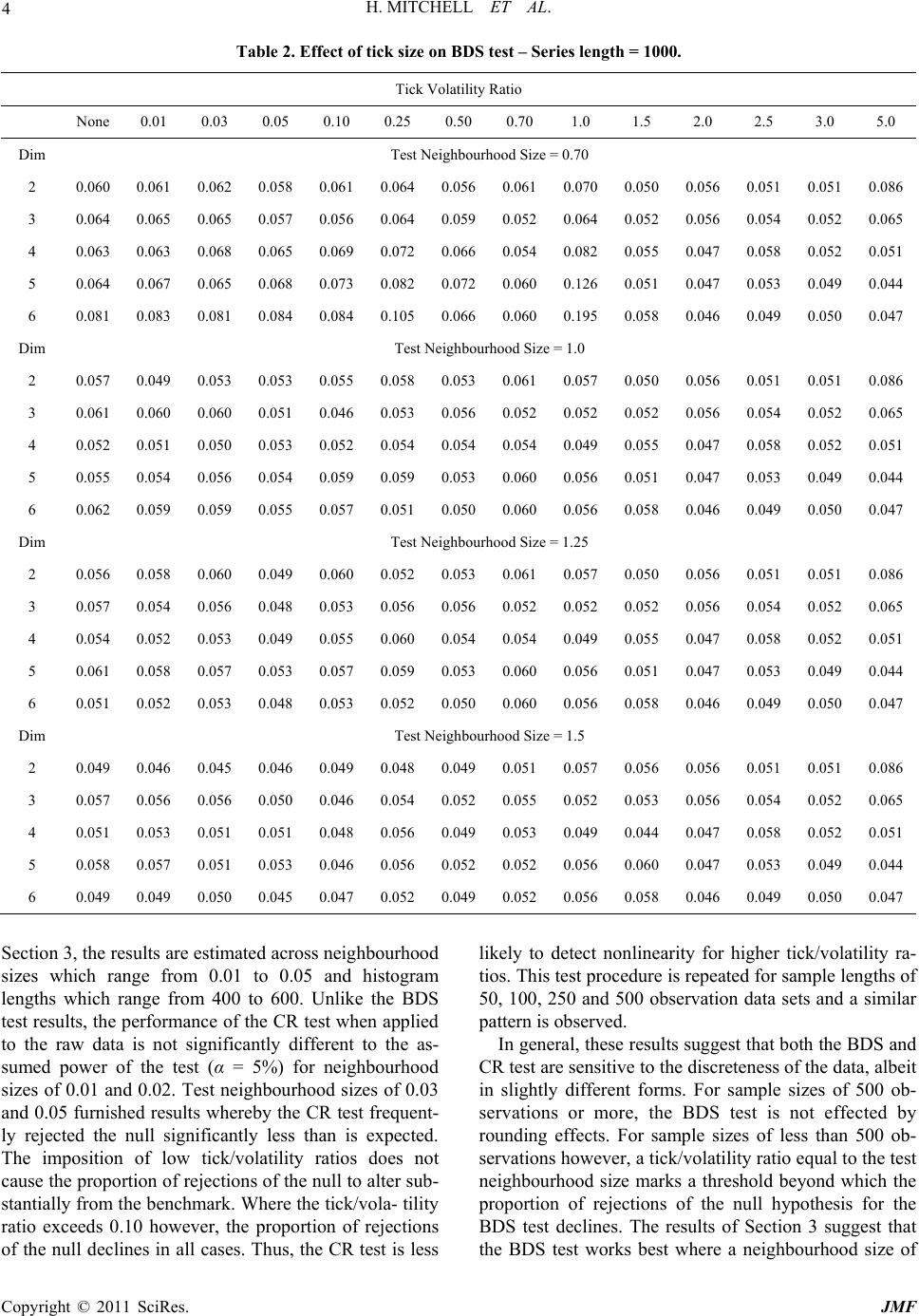

H. MITCHELL ET AL.
4
Table 2. Effect of tick size on BDS test – Series length = 1000.
Tick Volatility Ratio
None 0.01 0.03 0.05 0.10 0.25 0.50 0.70 1.0 1.5 2.0 2.5 3.0 5.0
Dim Test Neighbour hood Size = 0.70
2 0.060 0.061 0.0620.058 0.061 0.0640.0560.0610.0700.0500.056 0.051 0.0510.086
3 0.064 0.065 0.0650.057 0.056 0.0640.0590.0520.0640.0520.056 0.054 0.0520.065
4 0.063 0.063 0.0680.065 0.069 0.0720.0660.0540.0820.0550.047 0.058 0.0520.051
5 0.064 0.067 0.0650.068 0.073 0.0820.0720.0600.1260.0510.047 0.053 0.0490.044
6 0.081 0.083 0.0810.084 0.084 0.1050.0660.0600.1950.0580.046 0.049 0.0500.047
Dim Test Neighbourhood Size = 1.0
2 0.057 0.049 0.0530.053 0.055 0.0580.0530.0610.0570.0500.056 0.051 0.0510.086
3 0.061 0.060 0.0600.051 0.046 0.0530.0560.0520.0520.0520.056 0.054 0.0520.065
4 0.052 0.051 0.0500.053 0.052 0.0540.0540.0540.0490.0550.047 0.058 0.0520.051
5 0.055 0.054 0.0560.054 0.059 0.0590.0530.0600.0560.0510.047 0.053 0.0490.044
6 0.062 0.059 0.0590.055 0.057 0.0510.0500.0600.0560.0580.046 0.049 0.0500.047
Dim Test Neighbour hood Size = 1.25
2 0.056 0.058 0.0600.049 0.060 0.0520.0530.0610.0570.0500.056 0.051 0.0510.086
3 0.057 0.054 0.0560.048 0.053 0.0560.0560.0520.0520.0520.056 0.054 0.0520.065
4 0.054 0.052 0.0530.049 0.055 0.0600.0540.0540.0490.0550.047 0.058 0.0520.051
5 0.061 0.058 0.0570.053 0.057 0.0590.0530.0600.0560.0510.047 0.053 0.0490.044
6 0.051 0.052 0.0530.048 0.053 0.0520.0500.0600.0560.0580.046 0.049 0.0500.047
Dim Test Neighbourhood Size = 1.5
2 0.049 0.046 0.0450.046 0.049 0.0480.0490.0510.0570.0560.056 0.051 0.0510.086
3 0.057 0.056 0.0560.050 0.046 0.0540.0520.0550.0520.0530.056 0.054 0.0520.065
4 0.051 0.053 0.0510.051 0.048 0.0560.0490.0530.0490.0440.047 0.058 0.0520.051
5 0.058 0.057 0.0510.053 0.046 0.0560.0520.0520.0560.0600.047 0.053 0.0490.044
6 0.049 0.049 0.0500.045 0.047 0.0520.0490.0520.0560.0580.046 0.049 0.0500.047
Section 3, the results are estimated across neighbourhood
sizes which range from 0.01 to 0.05 and histogram
lengths which range from 400 to 600. Unlike the BDS
test results, the performance of the CR test when applied
to the raw data is not significantly different to the as-
sumed power of the test (α = 5%) for neighbourhood
sizes of 0.01 and 0.02. Test neighbourhood sizes of 0.03
and 0.05 furnished results whereby the CR test frequent-
ly rejected the null significantly less than is expected.
The imposition of low tick/volatility ratios does not
cause the proportion of rejections of the null to alter sub-
stantially from the benchmark. Where the tick/vola- tility
ratio exceeds 0.10 however, the proportion of rejections
of the null declines in all cases. Thus, the CR test is less
likely to detect nonlinearity for higher tick/volatility ra-
tios. This test procedure is rep eated for sample leng ths of
50, 100, 250 and 500 observation data sets and a similar
pattern is observed.
In general, these results suggest that both the BDS and
CR test are sensitive to the discreteness of the data, albeit
in slightly different forms. For sample sizes of 500 ob-
servations or more, the BDS test is not effected by
rounding effects. For sample sizes of less than 500 ob-
servations however, a tick/volatilit y ratio eq ual to th e test
neighbourhood size marks a threshold beyond which the
proportion of rejections of the null hypothesis for the
BDS test declines. The results of Section 3 suggest that
the BDS test works best where a neighbourhood size of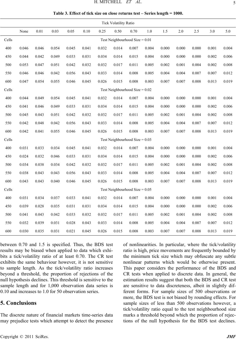

H. MITCHELL ET AL.
5
Table 3. Effect of tick size on close returns test – Series length = 1000.
Tick Volatility Ratio
None 0.01 0.03 0.05 0.10 0.25 0.50 0.70 1.0 1.5 2.0 2.5 3.0 5.0
Cells Test Neighbourhood Size = 0.01
400 0.046 0.046 0.0540.045 0.041 0.0320.0140.0070.0040.0000.000 0.000 0.0010.004
450 0.044 0.042 0.0490.033 0.031 0.0340.0140.0150.0040.0000.000 0.000 0.0020.006
500 0.053 0.047 0.0510.042 0.032 0.0320.0170.0110.0050.0020.001 0.004 0.0020.008
550 0.046 0.046 0.0420.056 0.043 0.0330.0140.0080.0050.0040.004 0.007 0.0070.012
600 0.047 0.054 0.0550.046 0.045 0.0260.0150.0080.0030.0070.007 0.008 0.0130.019
Cells Test Neighbourhood Size = 0.02
400 0.044 0.049 0.0540.045 0.041 0.0320.0140.0070.0040.0000.000 0.000 0.0010.004
450 0.041 0.046 0.0490.033 0.031 0.0340.0140.0150.0040.0000.000 0.000 0.0020.006
500 0.045 0.043 0.0510.042 0.032 0.0320.0170.0110.0050.0020.001 0.004 0.0020.008
550 0.042 0.048 0.0420.056 0.043 0.0330.0140.0080.0050.0040.004 0.007 0.0070.012
600 0.042 0.041 0.0550.046 0.045 0.0260.0150.0080.0030.0070.007 0.008 0.0130.019
Cells Test Neighbourhood Size = 0.03
400 0.031 0.033 0.0340.045 0.041 0.0320.0140.0070.0040.0000.000 0.000 0.0010.004
450 0.024 0.032 0.0460.033 0.031 0.0340.0140.0150.0040.0000.000 0.000 0.0020.006
500 0.034 0.038 0.0340.042 0.032 0.0320.0170.0110.0050.0020.001 0.004 0.0020.008
550 0.038 0.043 0.0430.056 0.043 0.0330.0140.0080.0050.0040.004 0.007 0.0070.012
600 0.043 0.043 0.0400.046 0.045 0.0260.0150.0080.0030.0070.007 0.008 0.0130.019
Cells Test Neighbourhood Size = 0.05
400 0.031 0.034 0.0370.033 0.041 0.0320.0140.0070.0040.0000.000 0.000 0.0010.004
450 0.039 0.028 0.0350.031 0.031 0.0340.0140.0150.0040.0000.000 0.000 0.0020.006
500 0.041 0.043 0.0420.033 0.032 0.0320.0170.0110.0050.0020.001 0.004 0.0020.008
550 0.032 0.039 0.0310.028 0.043 0.0330.0140.0080.0050.0040.004 0.007 0.0070.012
600 0.030 0.035 0.0310.021 0.045 0.0260.0150.0080.0030.0070.007 0.008 0.0130.019
between 0.70 and 1.5 is specified. Thus, the BDS test
results may be biased when applied to data which exhi-
bits a tick/volatility ratio of at least 0.70. The CR test
exhibits the same behaviour however, it is not sensitive
to sample length. As the tick/volatility ratio increases
beyond a threshold, the proportion of rejections of the
null hypothesis declines. This threshold is sensitive to the
sample length and for 1,000 observation data series is
0.10 and increases to 1.0 f or 50 observation seri es.
5. Conclusions
The discrete nature of financial markets time-series data
may prejudice tests which attempt to detect the presence
of nonlinearities. In particular, where the tick/volatility
ratio is high, price mov ements are frequen tly bounded by
the minimum tick size which may obfuscate any subtle
nonlinear patterns which would be otherwise present.
This paper considers the performance of the BDS and
CR tests when applied to discrete data. In general, the
estimation results suggest that both th e BDS and CR test
are sensitive to data discreteness, albeit in slightly dif-
ferent forms. For sample sizes of 500 observations or
more, the BDS test is not biased by rounding effects. For
sample sizes of less than 500 observations however, a
tick/volatility ratio equal to the test neighbourhood size
marks a threshold beyond which the proportion of rejec-
tions of the null hypothesis for the BDS test declines.

H. MITCHELL ET AL.
6
The CR test provides the same result however, it is not
sensitive to sample length. As the tick/volatility ratio
increases beyond a threshold, the proportion of rej ections
of the null hypothesis declines. This threshold is sensi-
tive to the sample length and for 1,000 observation data
series is 0.10 and increases to 1.0 for 50 observation series.
Tick/volatility ratios which exceed these thresholds
are frequently observed in financial markets data, which
suggests that the results of the BDS and CR test must be
interpreted with caution. Estimates of tick/volatility ra-
tios for exchange rate data range from 0.167 to 0.5 [36]
and for stock market range from 0.5 to 4.5 where prices
are quoted using decimals and 2.5 to 35 for those using
1/8ths [37]. Thus, financial markets data frequently exhi-
bit tick/volatility ratios which exceed the threshold
beyond which the BDS and pCR test are biased by the
discrete nature of pri ces.
6. References
[1] V. R. Anshuman and A. Kalay, “Market Making with
Discrete Prices,” The Review of Financial Studies, Vol.
11, No. 1, 1998, pp. 81-109. doi:10.1093/rfs/11.1.81
[2] C. Vorlow, “Stock Price Clustering and Discreteness: The
‘Compass Rose’ and Complex Dynamics,” Working Pa-
per, University of Durham, Durham, 2004.
[3] A. Antoniou and C. E. Vorlow, “Price Clustering and
Discreteness: Is There Chaos behind the Noise,” Physica
A, Vol. 348, 2005, pp. 389-403.
doi:10.1016/j.physa.2004.09.006
[4] C. Lee, K. Gleason and I. Mathur, “The Tick/Volatility
Ratio as a Determinant of the Compass Rose Pattern,”
European Journal of Finance, Taylor and Francis Jour-
nals, Vol. 11, No. 2, April 2005, pp. 93-109.
[5] H. Amilon, “GARCH Estimation and Discrete Stock Pri-
ces: An Application to Low-Priced Australian Stocks,”
Economics Letters, Vol. 81, No. 2, 2003, pp. 215-222.
doi:10.1016/S0165-1765(03)00172-1
[6] G. Gottleib and A. Kalay, “Implications of the Discrete-
ness of Observed Stock Prices,” Journal of Finance, Vol.
40, No. 1, 1985, pp. 135-154. doi:10.2307/2328052
[7] R. Koppl and S. Tuluca, “Random Walk Hypothesis Test-
ing and the Compass Rose,” Finance Letters, Vol. 2, No.
1, 2002, pp. 14-17.
[8] Y. Fang, “The Compass Rose and Random Walk Tests,”
Computational Statistics and Data Analysis, Vol. 39, No.
3, 2002, pp. 299-310.
doi:10.1016/S0167-9473(01)00063-9
[9] T. F. Crack and O. Ledoit, “Robust Structure without
Predictability: The Compass Rose Pattern of the Stock
Market,” Journal of Finance, Vol. 51, No. 2, 1996, pp.
751-762. doi:10.2307/2329379
[10] W. Kramer and R. Runde, “Chaos and the Compass
Rose,” Economics Letters, Vol. 54, No. 2, 1997, pp.
113-118. doi:10.1016/S0165-1765(97)00020-7
[11] W. Brock, W. Dechert and J. Scheinkman, “A Test for
Independence Based on the Correlation Dimension,”
Working Paper, University of Wisconsin, Madison, 1987.
[12] W. D. Dechert, “Testing Time Series for Nonlinearities:
The BDS Approach,” In: W. A. Kirman,et al., Eds. Non-
linear Dynamics and Economics: Proceedings of the 10th
International Symposium in Economic Theory and Eco-
nometrics, Cambridge University Press, Cambridge, 1996
[13] P. Grassberger and I. Procacia, “Measuring the Strange-
ness of Strange Attractors,” Physica D: Nonlinear Phe-
nomena, Vol. 9, No. 1-2, 1983, pp. 189-208.
[14] Y.-T. Chen and C.-M. Kuan, “Time Irreversibility and
EGARCH Effects in US Stock Index Returns,” Journal of
Applied Econometrics, Vol. 17, No. 5, 2002, pp. 565-578.
doi:10.1002/jae.692
[15] R. Ostermark, J. Aaltonen, H. Saxen and K. Soderlund,
“Nonlinear Modelling of the Finnihs Banking and Fi-
nance Branch Index,” European Journal of Finance, Vol.
10, No. 4, 2004, pp. 277-289.
doi:10.1080/13518470210124641
[16] R. T. Baillie, A. A. Cecen and Y.-W. Han, “High Fre-
quency Deutschemark-US Dollar Returns: FIGARCH
Representation and Non Linearities,” Multinational Fi-
nance Journal, Vol. 4, No. 3-4, 2000, pp. 247-268.
[17] C. G. Gilmore, “An Examination of Nonlinear Depend-
ence in Exchange Rates Using Recent Methods from
Chaos Theory,” Global Finance Journal, Vol. 12, No. 1,
2001, pp. 139-151. doi:10.1016/S1044-0283(01)00018-7
[18] V. Chwee, “Chaos in Natural Gas Futures?” The Energy
Journal, Vol. 19, No. 2, 1998, pp. 149-164.
doi:10.5547/ISSN0195-6574-EJ-Vol19-No2-10
[19] M. Frank and T. Stengos, “Chaotic Dynamics in Eco-
nomic Time Series,” Journal of Economic Surveys, Vol. 2,
No. 2, 1988, pp. 103-133.
doi:10.1111/j.1467-6419.1988.tb00039.x
[20] N. Kohzadi and M. S. Boyd, “Testing for Chaos and
Nonlinear Dynamics in Cattle Prices,” Canadian Journal
of Agricultural Economics, Vol. 43, No. 3, 1995, pp. 475-
484. doi:10.1111/j.1744-7976.1995.tb00136.x
[21] P. M. Bodman, “Steepness and Deepness in the Austra-
lian Macroeconomy,” Applied Economics, Vol. 33, No. 3,
2001, pp. 375-382. doi:10.1080/00036840122115
[22] C. G. Gilmore, “An Examination of Nonlinear Depend-
ence in Exchange Rates Using Recent Methods from
Chaos Theory,” Global Finance Journal, Vol. 12, No. 1,
2001, pp. 139-151. doi:10.1016/S1044-0283(01)00018-7
[23] C. G. Gilmore, “A New Test for Chaos,” Journal of Eco-
nomic Behaviour and Organisation, Vol. 22, No. 2, 1993,
pp. 209-237. doi:10.1016/0167-2681(93)90064-V
[24] C. G. Gilmore, “A New Approach to Testing for Chaos,
with Applications in Finance and Economics,” Interna-
tional Journal of Bifurcation and Chaos, Vol. 3, No. 3,
1993, pp. 583-587. doi:10.1142/S0218127493000477
[25] C. G. Gilmore, “Detecting Linear and Nonlinear De-
pendence in Stock Returns: New Methods Derived from
Chaos Theory,” Journal of Business and Finance Ac-

H. MITCHELL ET AL.
7
counting, Vol. 23, No. 9-10, 1996, pp. 1357-1377.
doi:10.1111/1468-5957.00084
[26] M. D. McKenzie, “Chaotic Behaviour in National Stock
Market Indices: New Evidence from the Close Returns
Test,” Global Finance Journal, Vol. 12, No. 1, 2001, pp.
35-53. doi:10.1016/S1044-0283(01)00024-2
[27] D. E. Knuth, “The Art of Computer Programming,” 3rd
Edition, Addison-Wesley Publishing Company, London.
1997.
[28] W. A. Brock, D. A. Hsieh and B. LeBaron, “Nonlinear
Dynamics, Chaos and Instability: Statistical Theory and
Economic Evidence,” MIT Press, London, 1991.
[29] P. L’Ecuyer, “Good Parameters and Implementations for
Combined Multiple Recursive Random Number Genera-
tors,” Operations Research, Vol. 47, No. 1, 1999, pp.
159-164. doi:10.1287/opre.47.1.159
[30] M. Matsumoto and T. Nishimura, “Mersenne Twister: A
623-Dimensionally Equidistributed Uniform Pseudo-Ran-
dom Number Generator,” ACM Transactions on Model-
ing and Computer Simulation, Vol. 8, No. 1, 1998, pp. 3-
30. doi:10.1145/272991.272995
[31] C. I. Lee, K. C. Gleason and I. Mathur, “A Comprehen-
sive Examination of the Compass Rose Pattern in Futures
Markets,” Journal of Futures Markets, Vol. 19, No. 5,
1999, pp. 541-564.
doi:10.1002/(SICI)1096-9934(199908)19:5<541::AID-F
UT3>3.0.CO;2-7
[32] E. Wang, R. Hudson and K. Keasey, “Tick Size and the
Compass Rose: Further Insights,” Economics Letters, Vol.
68, No. 2, 2000, pp. 119-125.
doi:10.1016/S0165-1765(00)00237-8
[33] D. Ruelle, “Deterministic Chaos: The Science and the
Fiction,” Proceedings of the Royal Society of London,
Vol. 427, No. 1873, 1991, pp. 241-248.
[34] J. B. Ramsay and H. J. Yuan, “Bias and Error Bars in
Dimension Calculations and Their Evaluation in Some
Simple Models,” Physics Letters A, Vol. 134, No. 5, 1989,
pp. 287-297. doi:10.1016/0375-9601(89)90638-5
[35] J. B. Ramsay and H. J. Yuan, “The Statistical Properties
of Dimension Calculations Using Small Data Sets,” Non-
linearity, Vol. 3, No. 1, 1990, pp. 155-175.
doi:10.1088/0951-7715/3/1/009
[36] K. C. Gleason, C. I. Lee and I. Mathur, “An Explanation
for the Compass Rose Pattern,” Economics Letters, Vol.
68, No. 2, 2000, pp. 127-133.
doi:10.1016/S0165-1765(00)00252-4
[37] M. D. McKenzie and A. Frino, “The Tick/Volatility Ratio
as a Determinant of the Compass Rose: Empirical evi-
dence from decimalisation on the NYSE,” Accounting
and Finance, Vol. 43, No. 3, 2003, pp. 331-344.
doi:10.1111/j.1467-629x.2003.00094.x