Engineering, 2011, 3, 435-444
doi:10.4236/eng.2011.35050 Published Online May 2011 (http://www.SciRP.org/journal/eng)
Sliding Mode Control, with Integrator, for a Class of
MIMO Nonlinear Systems
Anouar Benamor1, Larbi Chrifi-alaui2, Hassani Messaoud1, Mohamed Chaabane3
1Unit’e de Recherche en Automatique, Traitement du Signal et Image de l’ENIM, ATSI-ENIM, Monastir, Tunisie
2Laboratoire des Technologies Innovantes, Université de Picardie Jules Verne, Mitterrand, France
3Unité de Commande Automatique, l’Ecole Nationale d’Ingénieurs de Sfax, Sfax, Tunisie
Received January 24, 2011; revised March 8, 2011; accepted March 22, 2011
Abstract
In this paper, the robust control problem of general nonlinear multi-input multi-output (MIMO) systems is
proposed. The robustness against unknown disturbances is considered. Two algorithms based on the Sliding
Mode Control (SMC) for nonlinear coupled Multi-Input Multi-Output (MIMO) systems are proposed: the
first order sliding mode control (FOSMC) with saturation (sat) function and the FOSMC with sat combined
with integrator controller. Those algorithms were simulated and implemented on the three tanks test-bed
system and the experimental results confirm the effectiveness of our control design.
Keywords: Sliding Mode Control, Integrator, Nonlinear Systems, Coupled, Mimo, Uncertain, Liquid Level
Control
1. Introduction
The SMC is a widely used approach to design robust
control law of uncertain systems. The advantage of such
approach is its robustness to parameter variations and
disturbances [1,2]. But the major inconvenience of clas-
sic sliding mode control is the existence of chattering
phenomenon [3], which may induce many undesirable
oscillations in control signal. Some attempts on chatter-
ing [4] canceling have considered continuous functions
instead of sign one. However the provided results lead to
a large steady state error which can be reduced using the
integral action [5-7]. Moreover even though there exist
many works dealing with sliding mode control in the
case of Single Input Single Output (SISO) systems [8],
there is lock of results when the addressed process is
Multi-Input Multi-Output (MIMO) one. This shortage is
due to output coupling problem.
In this paper, we propose a first order sliding mode
control using Sat function and this control combined
with an integrator corrector. Experimental results, oper-
ated on a three tank system, are presented to illustrate the
effectiveness of the proposed controllers.
The paper is organized as follows. In Section 2 we re-
mind the classical sliding mode control of coupled MIMO
nonlinear systems and its robustness to parameter uncer-
tainties and external disturbances. Section three is de-
voted to SMC with sat function and integral action. The
model of the coupled three tanks system and its control is
presented in Section 4. The simulation and experimental
results are presented in Sections 5 and 6. Finally Section
7 concludes the paper.
2. Sliding Mode Control
Consider a MIMO non linear system with p inputs and m
outputs defined by the following state representation:



,,
,
x
fxtgxtu
ycxt
 





(1)
where x is the n-dimensional state vector and y is the
m-dimensional output vector.

1
T
n
x
xxand is the
m-dimensional vector, the coefficients of which are
nonlinear functions ci(x,t), f(x,t) is the n-dimensional
vector, the coefficients of which are nonlinear functions
fi(x,t), g(x,t) is a

1
T
m
yy y



pn

matrix with coefficients are the
nonlinear functions gij(x,t) and u is the p-dimensional
control vector of coefficients ui.

A. BENAMOR ET AL. 436


1
T
p
uu u    (2)
2.1. Classical Sliding Mode Control
Consider the sliding surface [9] defined by:
1
T
p
s
ss

 

(3)
where:
 
1
0
, for 1,,
i
r
ik
iki
k
s
ei 



p (4)
with:
ri is the relative degree of the error ei i and for
k = 1, , ri – 2,

11
i
r



i
k

are constants chosen so that
 
1
01 i
i
r
p 



k

ii
 1i
r


pis a Hurwitz polynomial one
and is the kth order derivative of the error ei.
i
e
, 1,,1.
d
iii i
eyyi r  (5)
where d
i
y
is the desired output. The derivative of si is:

1
01
de
d
i
rn
i
ii
k
kj
j
se
i
j
x
ttx














(6)
Replacing xj by its expression in (1) and omitting the
index (x,t), relation (6) becomes.

1
0111
d
d
i
rp
nn
i
iii i
kj
kjlj
jj
see e
jll
f
gu
ttxx




 



 

 (7)
which can be written as:
11
1
d
d
p
i
iiiP Piil l
l
shbubu hbu
t
 

 (8)
with:

1
01
i
rn
iii
ik
kj
j
ss
hf
tx











i
and

1
01
i
rn
ii
ik kjl
kj
j
s
bg
x










Then we can write the derivative of the surface vector as
s
hbu
 (9)
with:
111
1
and
P1
P
PP
hb
hb
hb
 
 

 
 
 


P
b
b

Theorem 1.
The control law for the first order sliding mode control
(FOSMC) of the system 1 so that the sliding surfaces go
to zero in a finite time is defined by:


11
1
PP
ksigns
ubh
ksigns







 









 (10)
with ki a positive constant and b an invertible matrix.
Proof.
Consider the following Lyapunov function:

2
1
11
22
T

2
P
Vss ss (11)
the derivative of V is:
11
T
PP
Vssss ss


(12)
Using (9) we have:


T
Vshbu
 (13)
Replacing u by its expression (10) in Equation (9), we
obtain:


11
PP
ksigns
s
ksigns











 (14)
then




11
11
0
pP
T
iii ii
ii
PP
ksigns
Vsksignss ks
ksigns 









(15)
Since ki (i = 1, , p) are positive we have V < 0. 
Then, the Lyapunov function V tends to 0 and there-
fore all surfaces si tend to zero, hence the existence of the
first order sliding mode.
To prove the finite time convergence of our control we
take the Equation (14), we have

ii ii
s
ksign ss
then
iii ii i
s
skss   
, with 0i
k

,which is the

reachability condition [10], then the finite time conver-
gence.
2.2. Robustness to Parametric Uncertainties and
External Disturbances
Consider an uncertain MIMO nonlinear system:



 


ˆˆ
,,,,
x
fxtfxtgxtgxtud

 
 (16)
where n x

is the state vector,
p
uis the input-
control bounded as maxii
uu for i = 1 to p, the vector
field




ˆ
,,

,
f
xtf xtfxt is continuous and
smooth, where


ˆ,
f
xt is the nominal part and


,
f
xt
is the uncertain part bounded by a known function.
n
dD


no
minal pa
represents the disturbances. The dynamic
g(t,x
the no
) is t exactly known an
rt
d it is written as the sum of


ˆ,
g
xt and the uncertain part


,
g
xt.

A. BENAMOR ET AL.437
with:
ˆ,



1
,
ˆ,
n
ˆ
f
xt
fxt
f
xt




,
 ˆ,



1
ˆ,
ˆ,
n
f
xt
fxt
f
xt






,

1
n
d
d
d
















 
11 1
1
ˆˆ
,,
ˆ,
ˆˆ ,,
P
nnP
g
xtg xt
gxt
g
xtgxt








and

 
 
11 1
1
,,
,
,,
P
nnP
g
xtg xt
gxt
g
xtgxt












Then the derivative of the sliding surface takes the
following form:

1
dˆˆ
d
p
i
i
sh
tiikik ki
k
hb bu


 
 (17)
then:


ˆˆ δ
shh bbu 




1
ˆ,
ˆ,
ˆ,
p
hxt
hxt
hxt






,



1,
,
,
p
hxt
hxt
hxt













,
1
δ
δ
δ
p













 
 
11 1
1
ˆˆ
,,
ˆ,
ˆˆ
,,
p
ppp
bxtb xt
bxt
bxtbxt









and


Theorem 2.
Consider the uncertain system defined by Equation
trol law:


(18)
with ki satisfying:
u (19)
and wher

 
 
11 1
1
,,
,
,,
p
ppp
bxtb xt
bxt
bxtbxt











(16). The con

1
ˆˆ
ksigns





11
PP
ub h
ksigns

 







*
max
1
δ
p
ii ikk
k




i
k
ei

, ik

,
ties,
te ti
*
δi
1
h,
e
and are
of uncertaiand respectively,
xpression of the derivative of the surface be-
maxk
u
ik
b, δi
rgenc
the upper bounds
n
fi
 
conve
k
ensures thenime of the sliding surface
to zero.
Proof.
The e
u
comes:

ˆˆ δshh bbu

 
 (20)
where s the p-dimensional vector wh
are :
δiose coefficients
1
δd for 1 to
n
i
s
ij
jj
ip
x




Using the control expression in (18) we ve: ha


11
ksigns 


δ
PP
sh
ks
igns
bu





 (21)
The derivative of the surface si is then written:

δ
ii i iikki
shksigns bu
1
p
k



 (22)
and the derivative of the Lyapunov function given by (12)
is:
1
ii
i
Vss

n


Veg

isfied
will be native if the following conditions are sat-
: 0ss
ii

 for i = 1 to p.
If si > 0 then 0
i
s , we have:
p
1
δ0
ik i
k
hk

iik
bu

   
 (23)
then
i
k
1
δ
p
iikki
k
hbu


 
 (24)
If si < 0 then 0
i
s

, we have:
1
δ0
p
i ki
k
h u

iik
k b

   
 (25)
then
i
k
1
δ
p
iikki
k
hbu



 


 (26)
The conditions (24) and (26) are satisfied if:
*
max δ ii kkii
uk 
1
p
k


 (27)
then
3. SMC with Sat
t of classic sliding mode control is
e existence of chattering phenomenon. To avoid this
0V

The major inconvenien
th

A. BENAMOR ET AL. 438
problem, we approximate the «sign» function by con-
tinuous functions such as sat function [9] defined by:
 
if
iii
sign ss
sat s if
ii
ii
i
ss






28)
where


 (
i

is a positive constant that defines the thickness
of the ary layer.
he first order sliding mode control
h sat of the system (1) is defined by:
bound
Theorem 3.
The control law for t
(FOSMC) wit


11
1
ksats
ubh





 

PP
ks ats









(29)
with ki a positive constant and b an invertible matrix.
Proof.
by
n (11). Its derivative with using control defined
in
We consider the same Lyapunov function defined
Equatio
(31) is:


ksats 

11
T
PP
Vs
ks ats

 




(30)
then
i
s (31)
Using sat definition given by (28), w

1
p
ii
i
Vksats




e have:


2
0 if
iii i
sign sss
0 if
ii i
ii
i
sat s sss






(32)
Therefore:
(33)
then
(34)
ark.
In the boundary layer the de



0
ii
satss
0V

Rem
rivative of the surface is:
i
i
i
s
s

 (35)
then

ee
ri ri
ii
tt tt
iiri i
sst




 (36)
with:
tri is the start time of boundary layer.
then
0 for 1,
iri ,
s
tt ip

  (37)
order to solve a steady-state error problem, an inte-
gral sliding manifold was proposed in [10]
op
(38)
with
In
. This devel-
ment is introduced and justified only by tests on spe-
cific systems. Our idea consists on reconstituting a con-
trol law to eliminate steady-state error created by distur-
bance. To do so we added an integral action when the
trajectories of states approach their references [11-14].
Proposition.
Consider the uncertain system defined by Equation (1).
aw FOSMC with integrator to eliminateThe control l
steady-state error is defined by:


11
1
d
d
yy t
ksats






 
11
11d
d
PP
ub h K
ksats yy t

   




 
 




11 1
1
p
p
pp
KK
K
KK














The coefficients Kij are the integrator constant defined
by:
j
j
p
ositive constant if >
d
ii
yy
0 if
ij d
ii
K
yy





(39)
with


j

a positive constant.
cription and Modeling
tem, which
ts on three
1
4. Validation
4.1. System Des
The considered process is a three tank sys
ave two inputs and three outputs. It consish
cylindrical tanks with identical Section a supplied with
distilled water, which are serially interconnected by two
cylindrical pipes of identical Sections Sn. The pipes of
communication between the tanks T1 and T2 are equipped
with manually adjustable valves; the flow rates of the
connection pipes can be controlled using ball valves az1
and az2. The plant has one outlet pipe located at the bot-
tom of tank T3. There are three other pipes each installed
at the bottom of each tank; they are provided with a di-
rect connection (outflow rate) to the reservoir with ball
valves bz1, bz2 and bz3, respectively, it can only be ma-
nipulated manually. The pumps 1 and 2 are supplied by
water from the reservoir with flow rates Q1(t) and Q2(t),
respectively. The necessary level measurements h(t),

A. BENAMOR ET AL. 439
oming flow and the outgoing
flo
h2(t) and h3(t) are carried out by the piezo-resistive dif-
ferential pressure sensors.
The state Equations are obtained by writing that the
variation of the water volume in a tank is equal to the
difference between the inc
12 1, 2, 3, 4
jzjL
BbSg j
A

While taking B1 = B2 = B3 = 0, the three Equations of
the system become (see Equation (44)):
At equilibrium, for constant water level set point, the
level derivatives must be zero.
ws, that means, the water of the tanks 1 and 2 can
flow toward the tank 3.
Then, the system can be represented by the following
Equations:
 

12
1 ,1,2,3
in outout
ii ijij
tQt Qt Qtij
123
0hhh


  (45)
Therefore, using (45) in the steady state, the
algebraic relationship holds.
following
h
A
 
 (40)

 
1
11313
=0
Q
csignh hh h


11 31333232
0
a
cs ignh hhhcsignhhhh


where s the flow through pump i (i = 1; 2) and
esents the flow rates of water betwee
, and can be expressed

in
i
Qti

repr
and j (,
e law o
1out
ij
Qt
tanks i
n the



(46)
For the coupled tanks system, the fluid flow Q1 into
tank 1, cannot be negative because the pump can
dr
From (47) we have
1,2,3 )iji j
using thf Torricelli[15].
 
1out
ijzii j
QtaS h i, j = 1, 3 (41)
and

2out
Qtrepresents the outfl
2
ni j
signhh gh
ow rate, given by:
only
ive water into the tank, then:
Q1 ≥ 0 (47)
ij

22 1, 2, 3 (42) out
ijzj Li
QtbSghj
e hi(t),

1
11 13
3
s ignh hh ha  and
Q
c
wher


in
i
Qtand


out
ij
Qt are respectively the
levels of t fle output
The parameters of three tank system are defi
ta
he system can be considered as a multi input
m
water, the inpuow and thflow rates.
ned in the
 
11313
signhh hh
3 3232
ccsignhh hh
Then (h1-h3) ≥ 0 and (h3-h2) ≥ 0. Therefore if we as-
sume.
Table 1.
The controlled signals are the water levels (h2, h3) of
nks 2 and tank 3. These levels are controlled by two
pumps. T 112 23 31122
, , , and
x
hxh xhuQuQ

  (48)
We h
ulti output system (MIMO) where the input are inflow
rates Q1, Q2 and the output are liquid levels h2, h3. Then
the three tank systems can be modeled by the following
three differential Equations as shown in (43):
where the parameters ci, i = 1, 3 and Bj, j = 1, 2, 3, 4 are
defined by:
ave
1
1113
2
2332 42
3113 332
u
xcxx
a
u
xcxxBxa
x
cxx cxx
 











(49)
12 1, 3
izin
caSg i
A


 
  
11
1131311
22
33232422
3
113133233323
d
d
d
d
d
d
hQ
csignhhh hBh
ta
hQ
csignh hh hBBh
ta
hcsign hhhhBBhcsign hhhh
t



2

(43)


 
11
11313
22
3323242
3
1131333232
d
d
d
hQ
csignhhhh
dt a
hQ
csignh hh hBh
dt a
hcsignhhhh csignhhhh
dt









(44)

A. BENAMOR ET AL. 440
which can be written in the same form of (1) as:

,
x
ftx gu
ycx



 (50)
where

123
T
x
xxx,

12
T
uuu,

23
T
yxx

11 3
33 42
113332
,ftxc xxB x
cx xcxx
cx x





 


 

,
10
a


1
0g  and
00
a





4.2. Sliding Mode Control of the Three Tank
System
The objective is to regulate the water levels of tank 2 and
tank 3 by using both laws defined in Section 3.
The vector of the sliding surface is given by:
010
001
c 


12
T
s
ss 
where:


122d
s
xx and

23333dd
s
xx xx  

x22 and
tank n be
written as follows:
2
d and x3d are the desired water levels of tank
3. The derivative of the sliding surface $s_1$ ca
11 12
s
lbu


 (51)
with:

 1332422d
lcxxBxx  and 1
12
ba


Similarly, the derivative of s2 is:
22211222
s
lbubu


 (52)
with:

11333211333242
221133323 1
1
2
d
lc xxcxxxc
x

 

3
3
2
xx 3
3 2
22
d
cxx cxxcxxcxx
c x
x
 
 

x B
22 3
1
2
bc
axx
 and 21 1
1
2
bc
axx

32 31
then
s
lbu
 (53)
ith:
an
ontrol SMC with sat vector is:
with:
w
1
2
l
ll



d b12
21 22
0b
bb



The C


1
1
22
ksign
ubl
ksign s


 






1
s 
(54)
313 2
cxx 




13
11
11 3 2
1
0
ac xxax x
c
b
a









Control SMC with integrator vector is defined by:


(55)
with:
The


11
11
1
22 22
()
()
d
d
yydt
ksigns
ubl K
ksigns yydt





 



 




11 12
21 22
KK
KKK







5. Simulation Results
The controllers designed in Section 3 are simulated using
the MATLAB software. The parameters of the three tank
system Figure 1 are given in Table 1.The paraeters for
the both controls for three tanks are
m
0.6

, k1= 0.699,
k2 = 0.53, K11 = 10−4, K12 = 18.10−3, K21 = 7.10−4 and K22
= −4
can notice that in the absence of chattering in controls u1
and u2 both controls proposed and both output h2
follows their desired references h2d and h3d.
ver, when we inject a disturbance at t = 1500 s in
low pipes of tank 2 and tank 3, the tow control-
lers ensure the convergence of the water levels h3 and h2
to their desired references h2d and 3d. We see in the
Figure 3 when we add integral action, the steady state
This is the advantage of the
-variables coupled system
case.
10 .
Simulation results are shown in Figures 2 to 4. We
and h3
Howe
the outf
h
error is almost eliminated.
controls proposed in multi

A. BENAMOR ET AL.441
a
z1
b
z4
h
2
h
3
h
1
b
z3
b
z1
b
z2
Cuve T
3
Cuve
Pomp 1
Q
1
Cuve T
2
Pomp 2
a
z2
Q
2
Figure 1. Three tank system.
0200 400 600 80010001200 1400 1600 1800 2000
0
0.05
0.1
0.15
0.2
Time ( sec )
Water level h
2
( m )
h
2
sat
h
2
d
h
2
sat+int
Zo om
Figure 2. Liquid level in tank 2.
1100 1200 13001400 15001600 17001800 19002000
0. 19
0. 195
0. 2
0. 205
0. 21
Ti me ( se c )
Wat er l evel h
2
( m )
Zoom
h
2
sat
h
2
d
h
2
sat+int
Figure 3. Liquid level with zoom in tank 2.
6. Experim
The proposed control algoithms were tested on the
physical laboratory plant (Figure 8) consisting of inter-
connected three tank system. The objective is to control
the liquid level of tanks 2 and 3. The experimental
schemes have been done under Matlab/Simulink, using
Real-Time Interface, and run on the DS1102 DSPACE
system, which is equipped by a power PC processor. The
control algorithm is implemented on DSP (TMS
320C31).
ental Results
r
0200 400 60080010001200 1400 1600 1800 2000
0
0.0 5
0.3 5
0. 1
0.1 5
0. 2
0.2 5
0. 3
er level h3 ( m )
Time ( sec )
Wat
h3sat
h3d
h3sat+int
Zoom
Figure 4. Liquid level in tank 3.
Table 1. Numerical values for physical parameters of the
three tank system.
SymbolValue Meaning
a 0.0154 m2 tank section
Sn 2.5 10−5 m2 cross-section of valve
aZi 01
zi
a

 flow correction term (i = 1, 2, 3)
zi
b 01
zi
b

 leakage flow correction term
(i = 1, 2, 3)
g 9.81 m/s2 gravity constant m/s2
hmax 0.6 m maximum water level in each tank
(i = 1, 2, 3)
Qimax 1.17 10−4 m3/smaximum inflow through pump i
(i = 1, 2)
1100 1200 1300 1400 1500 1600 1700 1800 1900
0.23
0. 32
0.27
5
0.24
0. 245
0.25
0. 255
0.26
0. 265
Time ( se c )
Wa
ter level h
3
( m )
h
3
sat
h
3
d
h
3
sat+int
Figure 5. Liquid level with z oom in tank 3.

A. BENAMOR ET AL. 442
0.22
Figure 6. Input signals of control Q1.
Figure 7. Input signals of control Q.
2
Figure 8. Real system. The parameters for both controls for
three tanks are: 

 ,
.10−5and
k1 = 0.46, k2 = 0.32, K11 = 10−3, K12
= 3.10−4, K21 = 11 K22 = 7.10−4.
For given references we remark that water levels h2d
and h3d reach their references without overshooting.
When we change the references we obtain the same re-
sponse. In order to test the robustness of our strate
with respecurbances,
gy
t to parameter uncertainties and dist
0200 400 600 8001000 1200 1400 1600 18002000
0.02
0.04
0.06
0.08
0.1
0.12
0.14
0.16
0.18
0.2
Wat er le v el h
2
( m )
Time ( sec )
h
2
d
h
2
sat+int
h
2
sat
Zoom
Figure 9. Liquid level in tank 2.
11001200 1300 140015001600170018001900 2000
0. 185
0. 19
0. 195
0. 2
0. 205
Time ( sec )
Water lev el h
2
( m )
h
2
d
h
2
sat+int
h
2
sat
Figure 10. Liquid level with zoom in tank 2.
we varied the parameters c1 and c3 by closing and open-
ing a little bit the valves az1 and az2 and we introduce a
permanent leakage in the outflow pipes of tank 2 and
tank 3 at t = the outflow
ipes of tank 2 and tank 3, the two controllers ensure the
convergence of the water level h3 and h2 to their desired
references h3d and h2d (Figures 9 and 11).
Then, the advantage of the sliding mode control with
integrator in simulation and experimental results is the
attenuation of error static (Figures 3, 5, 10, and 12).
Moreov er, we can also observe that control inputs Q1
and Q2 are smooth and the chattering phenomenon is
almost eliminated (Figures 6, 7, 13 and 14).
7. Conclusion
In this paper, robust sliding mode control for a class of
MIMO nonlinear systems was presented. In order
elimina state
rror inds slid-
g mode control, combined with a conditional integrator
1500 s. We remark at 1500 s in
p
to
te chattering phenomenon and the steady
uced by the use of sat function, continuoue
in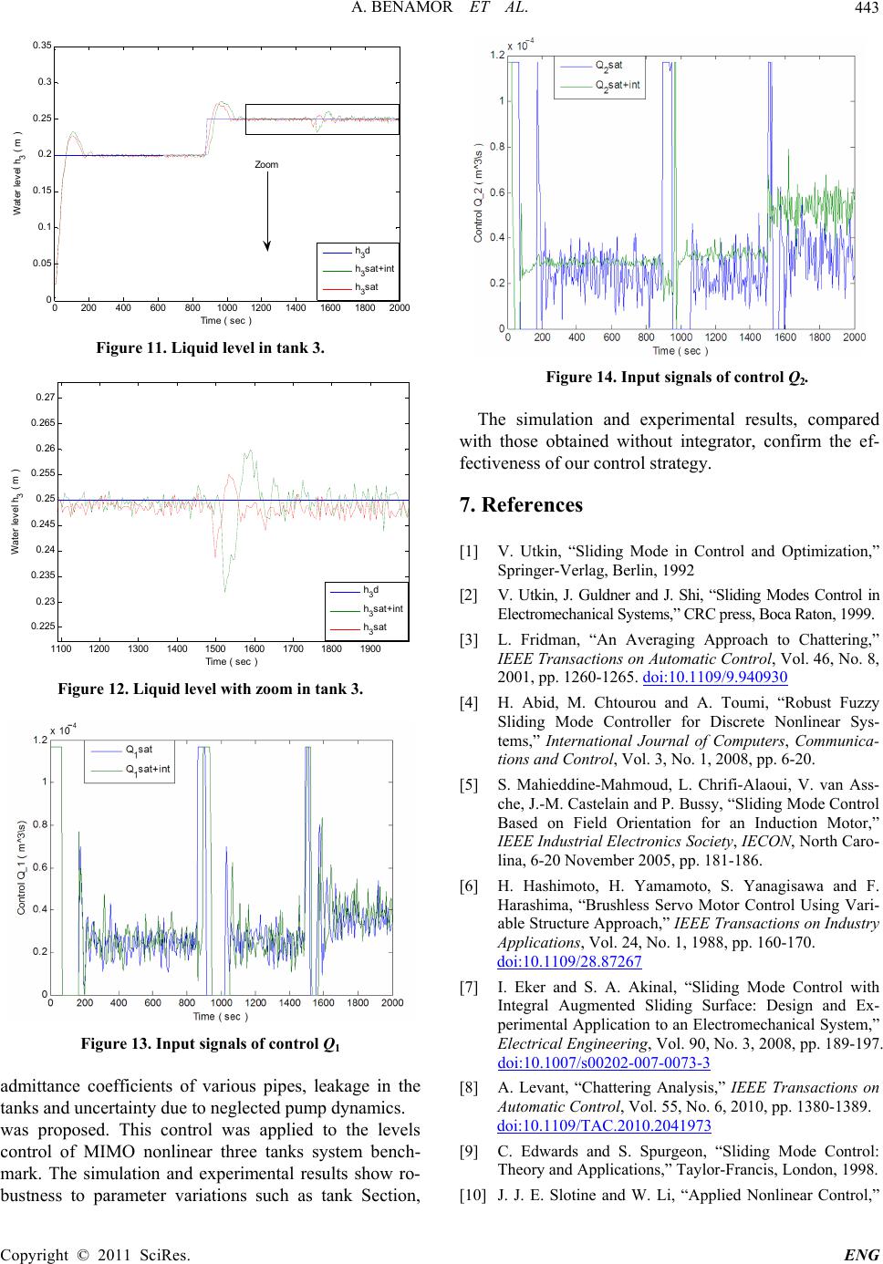

A. BENAMOR ET AL.443
0200 400 6008001000120014001600 1800 2000
0
0.05
0. 1
0.15
0. 2
0.25
0. 3
0.35
Time ( sec )
Wer level h
3
( m )
at
h
3
d
h
3
sat+int
h
3
sat
Zoom
Figure 11. Liquid level in tank 3.
11001200 1300140015001600 170018001900
0.225
0. 23
0.235
0. 24
0.245
0. 25
0.255
0. 26
0.265
0. 27
Time ( sec )
Water le
vel h
3
( m )
h
3
d
h
3
sat+int
h
3
sat
Figure 12. Liquid level with zoom in tank 3.
Figure 13. Input signals of control Q1
admittance coefficients of various pipes, leakage in the
tanks and uncertainty due to neglected pump dynamics.
was proposed. This control was applied to the level
control ench
ark. Tw ro-
ustness to parameter variations such as tank Section,
s
- of MIMO nonlinear three tanks system b
he simulation and experimental results shom
b
Figure 14. Input signals of control Q2.
[1] V. Utkin, “Sliding Mode in Control and Optimization,”
Springer-Verlag, Berlin, 1992
[2] V. Utkin, J. Guldner and J. Shi, “Sliding Modes Control in
Electromechanical Systems,” CRC press, Boca Raton, 1999.
[3] L. Fridman, “An Averaging Approach to Chattering,”
IEEE Transactions on Automatic Control, Vol. 46, No. 8,
2001, pp. 1260-1265. doi:10.1109/9.940930
The simulation and experimental results, compared
with those obtained without integrator, confirm the ef-
fectiveness of our control strategy.
7. References
[4] H. Abid, M. Chtourou and A. Toumi, “Robust Fuzzy
Sliding Mode Controller for Discrete Nonlinear Sys-
tems,” International Journal of Computers, Communica-
tions and Control, Vol. 3, No. 1, 2008, pp. 6-20.
[5] S. Mahieddine-Mahmoud, L. Chrifi-Alaoui, V. van Ass-
che, J.-M. Castelain and P. Bussy, “Sliding Mode Control
Based on Field Orientation for an Induction Motor,”
IEEE Industrial Electronics Society, IECON, North Caro-
lina, 6-
] H. Hashimoto, H. Yamamoto, S. Yanagisawa and F.
20 November 2005, pp. 181-186.
[6
Harashima, “Brushless Servo Motor Control Using Vari-
able Structure Approach,” IEEE Transactions on Industry
Applications, Vol. 24, No. 1, 1988, pp. 160-170.
doi:10.1109/28.87267
[7] I. Eker and S
Integral Augm
. A. Akinal, “Sliding Mode Control with
ented Sliding Surface: Design and Ex-
perimental Application to an Electromechanical System,”
Electrical Engineering, Vol. 90, No. 3, 2008, pp. 189-197.
doi:10.1007/s00202-007-0073-3
[8] A. Levant, “Chattering Analysis,” IEEE Transactions on
Automatic Control, Vol. 55, No. 6, 2010, pp. 1380-1389.
doi:10.1109/TAC.2010.2041973
[9] C. Edwards and S. Spurgeon, “Sliding Mode Control:
Theory and Applications,” Taylor-Francis, London, 1998.
[10] J. J. E. Slotine and W. Li, “Applied Nonlinear Control,”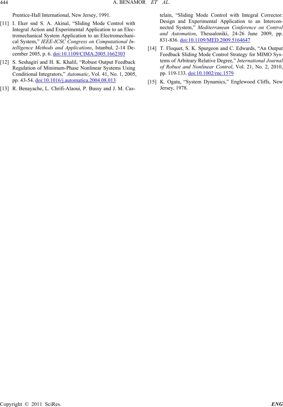

A. BENAMOR ET AL. 444
echani-
Prentice-Hall International, New Jersey, 1991.
[11] I. Eker snd S. A. Akinal, “Sliding Mode Control with
Integral Action and Experimental Application to an Elec-
tromechanical System Application to an Electrom
cal System,” IEEE-ICSC Congress on Computational In-
telligence Methods and Applications, Istanbul, 2-14 De-
cember 2005, p. 6. doi:10.1109/CIMA.2005.1662303
[12] S. Seshagiri and H. K. Khalil, “Robust Output Feedback
Regulation of Minimum-Phase Nonlinear Systems Using
Conditional Integrators,” Automatic, Vol. 41, No. 1, 2005,
pp. 43-54. doi:10.1016/j.automatica.2004.08.013
[13] R. Benayache, L. Chrifi-Alaoui, P. Bussy and J. M. Cas-
telain, “Sliding Mode Control with Integral Corrector:
Design and Experimental Application to an Intercon-
nected System,” Mediterranean Conference on Control
and Automation, Thessaloniki, 24-26 June 2009, pp.
831-836. doi:10.1109/MED.2009.5164647
[14] T. Floquet, S. K. Spurgeon and C. Edwards, “An Output
Feedback Sliding Mode Control Strategy for MIMO Sys-
tems of Arbitrary Relative Degree,” International Journal
of Robust and Nonlinear Control, Vol. 21, No. 2, 2010,
pp. 119-133. doi:10.1002/rnc.1579
[15] K. Ogata, “System Dynamics,” Englewood Cliffs, New
Jersey, 1978.