International Journal of Geosciences, 2011, 2, 172-178
doi:10.4236/ijg.2011.22018 Published Online May 2011 (http://www.SciRP.org/journal/ijg)
Land Use and Land Cover Change (LULC) in the Lake
Malawi Drainage Basin, 1982-2005
Geoffrey Chavula1*, Patrick Brezonik2, Marvin Bauer3
1University of Malawi–The Polytechnic, Blantyre, Malawi
2Department of Civil Engineering, University of Minnesota, Minneapolis, USA
3Department of Forest Resources, University of Minnesota, Saint Paul, USA
Received March 16, 2011; revised April 18, 2011; accepted May 10, 2011
Abstract
Changes in land use and land cover (LULC) in the drainage basin of Lake Malawi over the period 1982 -
2005 were estimated from satellite imagery, and possible relationships were evaluated among the four major
land-cover classes: cropland, forest, water, and savanna/shrub/woodland. AVHRR and MODIS sensors gave
different values of areal extent of the four classes, limiting the feasibility of establishing consistent temporal
trends over the entire period of the study, but forest land showed the least change among three land cover
types, and extent of water bodies remained virtually unaltered over the period. AVHRR results show that
cropland was mainly derived from savanna/shrub/woodland, which declined by almost 90% over the period
1982-1995.
Keywords: AVHRR, Lake Malawi, Lake Surface Temperature, MODIS, Reflectance
1. Introduction
Deforestation and agricultural production in the drainage
basin of Lake Malawi have the potential to cause water
quality deterioration that could impact the lake’s rich
biodiversity. Runoff from agricultural lands may increase
loadings of suspended solids and nutrients to the lake,
and rises in lake levels may be caused by reductions in
interception and evapotranspiration when forests are con-
verted to cropland. Forests intercept a large proportion of
the rainfall, much of which is lost to the atmosphere
through evapotranspiration. Forests transpire more water
than crops, and these processes thus reduce surface run-
off in forest environments.
According to Malawi’s National Environmental Ac-
tion Plan (NEAP) of 1994, rapid expansion of agricul-
tural production from the mid-1970s to late 1980s re-
sulted in extensive deforestation [1]. The rate of defores-
tation was 3.5% per annum during that period, but it de-
clined to 1.6% by 1994 because little forested land was
left. Additional deforestation was caused by use of wood
fuel for tobacco curing, cooking, and domestic heating.
Deforestation in the drainage basin of Lake Malawi may
be similar to the national picture presented by the NEAP
because the basin covers more than half of the country’s
total area. Detailed studies have not been reported on
which land-cover class(es) contributed to the creation of
cropland nor to confirm that depletion of forests led to
increased cropland area.
The primary objectives of this study were to assess
land-use and land-cover change (LULC) in the Lake
Malawi drainage basin over the period 1982 - 2005 and
to evaluate the source of new cropland. We used a com-
bination of AVHRR and MODIS satellite imagery be-
cause the more sophisticated MODIS data were not
available for much of the timeframe of interest. A sec-
ondary objective was to assess the comparability of LU-
LC results obtained from the two imagery sources.
2. Lake Malawi Drainage Basin
Lake Malawi is the third largest lake in Africa, and is
located at the border between Malawi, Mozambique and
Tanzania (Figure 1). Figure 1 shows the areal extent of
the Lake Malawi Basin, depicted by the satellite imagery,
with the lake’s tributaries shown as solid lines and the
boundary of the basin marked by dashed lines. The dia-
mond dots represent ground observation points recorded
during the field research aimed at verifying land use and
land cover classes noted during the classification process.

G. CHAVULA ET AL.173
TANZANIA
TANZANIA
MOZAMBIQUE
ZAMBIA
MOZAMBIQUE
MALAWI
Lillongwe
N
♦
♦
♦
♦
♦
♦
♦
♦
♦
♦
♦
♦
♦
♦
♦
♦
♦
♦
♦
♦
♦ ♦
♦
♦♦
♦
♦
♦
♦
♦
♦
♦
♦
♦
♦
♦
♦
♦
050 km
Shire
River
Figure 1. Map of Lake Malawi and its drainage basin with
location of ground observation points shown as black dia-
monds.
These points appear as red dots on the satellite imagery.
The northern two-thirds of the Lake Malawi drainage
basin are a mixture of evergreen (Braschystegia) wood-
lands and agriculture [2]. The southern third is woodland
in Mozambique but almost completely cultivated in Ma-
lawi. The drainage basin has a higher population density
(100 km−2) than that of Lake Tanganyika (33 km−2) but
lower than that of Lake Victoria (up to 1200 km−2) [3].
The rapidly growing population in the Lake Malawi ba-
sin is sustained by small-scale agriculture, which causes
increasing stress on the land, as increasingly marginal
lands with steep slopes are brought into production [3,4].
Water levels of Lake Malawi have varied widely over
the period of continuous record [5]. The lake reached its
lowest level, 469.94 m above mean sea level (MSL), in
1915, and outflow to the Shire River ceased until 1935.
High lake levels occurred during 1979 - 1984, and a re-
cord rise (1.83 m) during 1978 - 1979 caused serious
flooding of coastal areas and the Lower Shire Valley.
Calder et al. [6] concluded from model simulations that
rainfall variations alone were responsible for water level
fluctuations from 1896 to 1967 but that a 13% depletion
of forest-cover in the basin during 1967 - 1990 led to an
increase in lake level. They concluded that if forest de-
pletion not had occurred, the lake’s water level would
have been 1 m lower. In this respect, removal of forests
from the basin saved the country from experiencing se-
rious consequences from the 1991/92 drought.
During periods of heavy storms, rising lake levels trig-
ger flooding in coastal areas and the Lower Shire Valley
compounding the severity of flooding in the Zambezi
River in Mozambique, downstream of the Shire River
confluence [5,7]. The lake level also has implications for
sustainability of hydropower plants in the Shire River,
which generate ~284 MW. They were developed after a
flow-control structure was constructed in 1965 at Li-
wonde (the Kamuzu Barrage) to maintain the lake at
473.2 - 475.32 m MSL and maintain a river flow of
~170 m3/s [5]. Higher flows and levels could damage the
structure.
3. LULC Classification Using Satellite
Imagery
The procedure for determining changes in LULC using
satellite imagery begins with selecting the phenomenon
to represent change [8]. The following steps are then
used to analyze the phenomenon: image acquisition, im-
age preparation, selection of a change detection algo-
rithm, and production of change detection results. Image
preparation includes selecting images and eliminating
interferences in them. Change detection involves either
bi-temporal or trend analysis [8]. The former compares
images from two discrete times, and the latter evaluates
change based on data for multiple dates from a time se-
ries of images. Normally, anniversary dates are used for
bi-temporal change detection to minimize effects of
phenological cycles and sun angle.
Coppin et al. [9] grouped change-detection algorithms
into eleven categories, and Coppin and Bauer [10] con-
cluded that image differencing, PCA, and the mul-
ti-temporal Kauth-Thomas methods perform better than
other approaches. As stressed by Jensen [11], the major
assumption in change detection is that a difference exists
in the spectral characteristics of a pixel on two dates if
biophysical conditions in the pixel field changed between
dates.
Vegetation indices often are used as empirical meas-
ures of vegetation status [12]. Many studies have dem-
onstrated relationships between red and near-infrared
(NIR) reflected energy and the amount and type of vege-

G. CHAVULA ET AL. 174
tation on the ground [13]. According to Huete et al. [12],
reflected red energy decreases with plant development
because of absorption by chlorophyll in actively photo-
synthetic leaves, and reflected NIR energy increases
through scattering processes in healthy leaves. A com-
mon vegetation index is the NDVI (normalized differ-
ence vegetation index):
tral matching techniques (SMTs), followed by class iden-
tification and merging using ground observations, Goo-
gle Earth imagery, and other secondary data to produce
maps of LULC classes for each year of data [14,15].
Areal coverage by LULC class was used to measure
changes over the period 1982-2005. Two SMT variations
were used to classify LULC change—spectral correlation
similarity (SCS) and spectral similarity value (SSV).
Thenkabail et al. [16] showed that both are useful in
classifying LULC types.


NDVI nir red
nir red
XX
XX

 (1)
SCS is based on Pearson’s correlation coefficient (r)
applied to an NDVI time series [14]:
The NDVI may range in value from −1.0 to +1.0. A
value of +1 indicates healthy vegetation; values close to
zero indicate poor vegetation. Tropical forests show little
intra-annual variation in NDVI, but rain-fed crops ex-
hibit strong seasonality. Temporal signatures of NDVI
vary according to vegetation type, and this is used to
identify land-cover type (e.g., distinguish between forest
and crop land).
 
1
1
1
n
itih
i
th
th
rn


















(2)
where ti = NDVI time series of the target class; μt = mean
of the NDVI time series of the target class; hi = NDVI
time series of any other class; μh = mean of the NDVI
time series of any class; σt = standard deviation of target
class NDVI time series; and σh = standard deviation of
NDVI time series of other class. Although r can range
from −1.0 to +1.0, negative values are not meaningful
here [14]. The higher the value of r, the greater the simi-
larity of the spectral or temporal NDVI profile between
the historical and recent time series land-use and land-
-cover class [15].
4. Methods
The following datasets were used to conduct the analysis
of LULC change: 8-km resolution AVHRR-NDVI data
for 1982 - 2000 and MODIS 7-Band Reflectance Data
for 2000 - 2005, converted to NDVI (Table 1). In addi-
tion, we used Lake Malawi water level data from the
Malawi Ministry of Irrigation and Water Development,
Hydrology Section Data Archive, for the period 1982 -
2005 and ground observations for major land use and
land-cover classes for the Lake Malawi basin, as well as
Google Earth imagery, existing land use and land cover
maps, and topographic maps.
SSV was defined by Homayouni and Roux [16] as:

2
2
SSVEDS1 r (3)
LULC analysis was done using the method of Thenk-
abail et al., which involves class development byspec-
where EDS is the Euclidian distance between the histori-
cal LULC class and a recent LULC class in spectral
Table 1. Datasets used for LULC change in Lake Malawi drainage basin.
Satellite Sensor and Band Wavelength (µm) Data Format Range
AVHHR (8 km)
Band 1 (B1) 0.58 - 0.68 Reflectance at ground, 8-bit 0 - 100%
Band 2 (B2) 0.73 - 1.10 Reflectance at ground, 8-bit 0 - 100%
Band 4 (B4) 10.3 - 11.3 Brightness temperature
(top of atmosphere) 160 - 340
Band 5 (B5) 11.5 - 12.5 Brightness temperature
(top of atmosphere) 160 - 340
NDVI (B2 – B1)/(B2 + B1) No units, 8-bit scaled NDVI –1 to +1
MODIS/Terra
7-Band-500 m reflectance data
processed to NDVI (B2 – B1)/(B2 + B1) No units; 16-bit scaled NDVI –1 to +1

G. CHAVULA ET AL. 175
space [15]. SSV was used to match both the shape and
magnitude of the classes. The Euclidian distance EDS is
given by:

2
1
EDS
n
ii
i
tr


 (4)
The typical range of SSV is 0 - 1.415; smaller values
indicate greater similarity.
Monthly data on the maximum-value composite NDVI
for AVHRR were downloaded for the Lake Malawi ba-
sin from the International Water Management Institute
Data Support Pathway (IWMI DSP) archive for 1982 -
1995; and maximum composite NDVI values for MOD-
IS/Terra were calculated for the Lake Malawi basin from
7-Band Reflectance Data of bands 1 and 2 for 2000 - 2005
using ERDAS Imagine and ER Mapper computer pack-
ages. The cloud removal algorithm of Thenkabail et al.
[14] was not used because we assumed that the compos-
ite NDVI values eliminated cloud interference by making
use of at least one cloud-free day in computing the data
series.
Unsupervised land cover classification was carried out
on the NDVI series by the ISODATA routine in ERDAS
Imagine, which calculates class means evenly distributed
in the data space and clusters the remaining pixels itera-
tively using a minimum distance technique. Initially, 50
classes were defined, from which NDVI was plotted
versus month for the period 1982 - 2000. Spectral
matching by SCS then was used to group signatures rep-
resenting similar classes. The process started by group-
ing classes with r2 > 0.96, followed by 0.92 < r2 < 0.96,
0.90 < r2 < 0.92, 0.85 < r2 < 0.90, and finally r2 < 0.85.
The choice of r2 ranges was made based on previous ex-
perience with LULC classification. In each range, signa-
tures were classified further into smaller groups depend-
ing on similarity of the NDVI signatures. After merging,
further grouping was done with the assistance of ground
observation photos, Google Earth, the USGS
land-use/land- cover map, Global Land Cover (GLC)
2000 land-use/ land-cover map, and the Malawi Depart-
ment of Surveys draft LULC map. A single class was
assigned to each 8 km  8 km pixel in AVHRR images
and each 0.5 km  0.5 km pixel in MODIS images after
examining the accessory information. Finally, four
classes were obtained: water bodies, cropland, evergreen
forests, and savanna/ shrubs/woodland (SSW).
For both AVHRR and MODIS images, verification of
the identified classes was done using geo-linked land-
use/land-cover maps (USGS, GLC), Landsat and Google
Earth imagery, and ground observation photos. Pixels
falling in the “wrong” category were cropped out of the
image and placed in the appropriate class. For example,
several pixels falling in the cropland, SSW, or forest
categories found in Lake Malawi in the analyses of
MODIS images were cropped out and placed under “wa-
ter bodies.”
Ground observations were made for the LULC classes
at specific locations in the Lake Malawi basin, shown in
Figure 1 as diamond dots and red dots on the satellite
imagery. A Garmin GPS unit was used to locate the
ground observation points. Collection of ground-based
calibration data for the LULC classification focused on
dominant classes, namely: evergreen forests; patches of
natural woodlands (including Miombo); grassland; shrub
and scrub land; “dambos” (i.e. , wetlands in the plateau
area); and farmland, including home gardens. Collection
of calibration data involved travel to basin areas where
these classes were thought to occur. This approach dif-
fers from the common approach to collect ground obser-
vation data—sampling on a uniform length scale (e.g.,
every 10 km of road travel), which would not have been
useful because most of the land in the basin falls in the
cropland class.
5. Results and Discussion
A wide variety of patterns occurred in monthly values of
NDVI calculated from 2001 MODIS data among the
50-unsupervised LULC classes extracted by ERDAS
ISODATA. The variations of NDVI of the 50 classes
with time in months are shown in Figure 2(a); but many
classes of LULC did exhibit substantial similarity. For
example, classes 17, 19, and 26 shown in Figure 2(b)
were merged into one group because their correlation
coefficient was greater than 0.96, i.e., SCS of r2 > 0.96.
Figures 2(a) and 2(b) illustrate transitional results ob-
tained in the classification process before the four final
LULC classes were identified, namely: water bodies,
cropland, evergreen forests, and savanna/shrubs/wood-
land (SSW).
Spatial distributions of the final four LULC classes
over the study period are shown in Figure 3 (8-km reso-
lution AVHRR-NDVI data for 1982, 1985, 1990, and
1995) and Figure 4 (0.5 km resolution MODIS-NDVI
data for 2001 and 2005). Inspection of the areal extent
data for each LULC class over the six years (Table 2)
shows that the two sensors yielded discordant results
regarding areal extents of the classes and changes in
LULC in the Lake Malawi basin over the period of anal-
ysis. Consequently, it is more instructive to consider the
two image sources separately.
For AVHRR, forest area decreased by ~25% initially
(1980 to 1985) and then increased gradually during the
period 1985 - 1995 such that the extent of forest in 1995
was within 91% of the initial value. The area of cropland
nearly doubled between 1982 and 1985 but then re-

G. CHAVULA ET AL. 176
Figure 2. (a) NDVI versus month for 50 classes produced by unsupervised classification for 2001 MODIS data; (b) plots for
three of the classes with SCS R2 > 0.96.
mained relatively constant. In contrast, the area of sa-
vanna/shrub/woodland (SSW) decreased dramatically,
especially between 1982 and 1985, and by 1990 the ex-
tent of SSW was only 13% of the 1982 value. The results
indicate that cropland area increased primarily at the
expense of SSW. The area of surface water remained
fairly constant over the period of AVHRR data, although
it increased by ~9% between 1990 and 1995. For MOD-
IS, forested and water areas were fairly constant between
the two years of data, but cropland decreased and SSW
increased by similar amounts. Thus cropland and SSW
again appear to be interchangeable.
Analysis of LULC data from the two sensors yielded
moderate differences in areal extent for forested land,
with the MODIS imagery yielding about a third more
forest than the AVHRR imagery. The two sensors
yielded even larger differences in extent for cropland and
SSW, but they did agree on the areal extent of surface
water, which essentially represents Lake Malawi. The
differences in areal coverage for the three land classes
likely can be attributed to differences in spatial resolu-
tion of the sensors. Much more class-averaging occurs

G. CHAVULA ET AL.177
Figure 3. Distribution of the four LULC classes in Lake
Malawi basin from AVHRR imagery for (a) 1982, (b) 1985,
(c) 1990, and (d) 1995.
Figure 4. Distribution of the four LULC classes in Lake
Malawi basin from MODIS imagery for (a) 2001 and (b)
2005.
with the AVHRR data, given its low (8 km) resolution,
than with the MODIS data. Hence, small differences
between classes are more likely to be distinguishable
using MODIS than AVHRR data. Because surface water
in the basin occurs mostly in one large water body, av-
eraging of within-pixel spectral characteristics is much
less an issue for this class than for spatially heterogene-
ous land classes.
The temporal changes in LULC areal coverage (Table
2) show no obvious relationship between forest depletion
and lake level rise. From the AVHRR data, it appears
that there was a small net decrease in forests between
1982 and 1995 (<9%), but the lake level decreased by
2.4 m. The MODIS data show a small (3%) decease in
the extent of forests from 2001 to 2005, but the lake level
rose by 0.3 m. The differences in areal coverage of forest
between the two sensors preclude combining the data to
examine relationships between water level and forest
over the entire study period.
The results in Table 2 indicate that SSW lands rather
than forests have suffered the most serious depletion in
the Lake Malawi basin as cropland has expanded and
agricultural production has increased. These findings
contrast the results of Calder et al. [6], who concluded
that forest depletion in the basin of Lake Malawi caused
an increase in lake level. Although evapotranspiration
may not be as high in SSW as in forests, because rainfall
interception by broad leaves of the evergreen forests is
generally high and thus associated evaporation losses are
also high and accentuated by eddies generated by wind
blowing over the forest stand, the increase in surface
runoff that likely results from converting SSW to crop-
land nonetheless has the potential to increase the lake
level.
Most of the Lake Malawi Basin is covered by SSW
hence it is not surprising that cropland is mainly from
this LULC class. The other reason for this scenario is
that areas where forests occur in the Lake Malawi Basin
are sparsely populated. Thus, there is very little effect on
forest cover with the encroachment of human activities
such as agricultural production. But this situation is be-
ing to change in future as more people in Malawi move
into forest areas in search of prime land for settlement
and agricultural production, especially tobacco and ma-
ize production.
The differences between the AVHRR and MODIS da-
ta for areal extent of the LULC classes were unexpected,
but upon reflection the differences do make sense
Table 2. Areal extent of LULC classes (in km2), and lake level (m above sea level) in Lake Malawi drainage basin.
Year Imagery Forest Cropland Water Bodies SSW1 Lake Level
1982 AVHRR 26 741 45 738 29 040 43 681 476.05
1985 AVHRR 20 086 86 273 28 193 10 648 475.17
1990 AVHRR 22 264 87 846 29 403 5 687 475.42
1995 AVHRR 24 442 83 490 31 944 5 324 473.66
2001 MODIS 33 800 46 408 29 707 20 091 474.51
2005 MODIS 32 739 40 545 29 799 26 921 474.83
1SSW = savanna/shrub/woodlands.

G. CHAVULA ET AL. 178
given the large difference in spatial resolution between
the two sensors and the patchy nature of land cover in
Malawi. Because of the short temporal extent (2001 -
2005) of MODIS data, our analysis of temporal trends is
based primarily on the AVHRR data. If we had been able
to use 1-km AVHRR-NDVI data instead of 8-km resolu-
tion data, the inferred LULC distributions may have been
more compatible with the MODIS results, but such data
were not available.
6. Conclusions
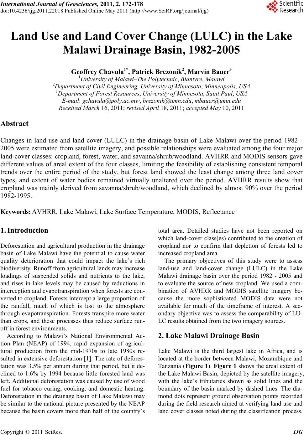
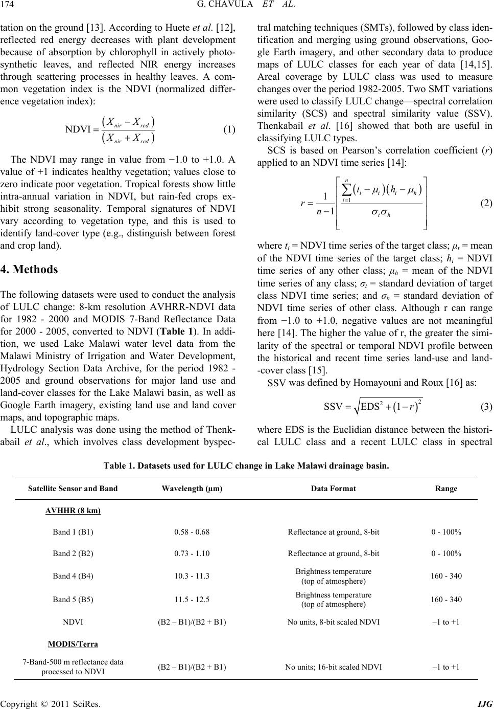
Because of differences in spatial resolutions, AVHRR
and MODIS sensors gave different values for areal ex-
tent of the forest, cropland and SSW land classes over
the period of analysis. The extent of surface water re-
mained virtually unchanged over the period 1982 - 2005.
Both the AVHRR and the MODIS data show that crop-
land was mainly derived from SSW.
7. Acknowledgements
The authors thank the International Water Management
Institute (IWMI), University of Minnesota, and START
for funding for the study. Use of the facilities of the Re-
mote Sensing Laboratory and Water Resources Center at
the University of Minnesota and Monkey Bay Fisheries
Research Station in Malawi is greatly appreciated. We
are happy to acknowledge technical support from James
Kuyper, NASA; John Sapper, NOAA; Ye Myint, Leica;
Prasad Thenkabail, USGS; and the Ministry of Irrigation
and Water Development in Malawi.
8. References
[1] Environmental Affairs Department, “National Environ-
mental Action Plan,” Malawi Government, Lilongwe,
1994.
[2] H. A. Boostma and R. E. Hecky, “Conservation of the
African Great Lakes: A Limnological Perspective,” Con-
servation Biology, Vol. 7, No. 3, 1993, pp. 644-656.
doi:10.1046/j.1523-1739.1993.07030644.x
[3] H. Bootsma and S.E. Jorgensen, “Lake Malawi/Nyasa,”
2004.
http://www.worldlakes.org/uploads/ELLB%20Malawi-N
yasaDraftFinal.14Nov2004.pdf
[4] F. X. Mkanda, “Contribution by Farmer’s Survival Strat-
egies to Soil Erosion Strategies in the Linthipe River
Catchment: Implications for Biodiversity Conservation in
Lake Malawi/Nyasa,” Biodiversity and Conservation,
Vol. 11, No. 8, 2002, pp. 1327-1359.
doi:10.1023/A:1016265715267
[5] O. N. Shela, “Naturalization of Lake Malawi Levels and
Shire River Flows: Challenges of Water Resources Re-
search and Sustainable Utilization on the Lake Malawi –
Shire River System,” Water Net Symposium: Sustainable
Use of Water Resources, Maputo, 1-2 November 2000,
pp. 1-12.
[6] I. R. Calder, R. L. Hall, H. G. Bastable, H. M. Gunston,
O. Shela, A. Chirwa and R. Kafundu, “The Impact of
Land Use Change on Water Resources in the Sub-Saha-
ran Africa: A Modeling Study of Lake Malawi,” Journal
of Hydrology, Vol. 170, No. 1-4, 1995, pp. 123-135.
doi:10.1016/0022-1694(94)02679-6
[7] S. S. Chiotha, G. M. S. Chavula, S. Chikwembani, E. B.
Khonga and E. Y. Sambo, “National Disaster Manage-
ment Plans for Malawi,” Ministry of Disaster, Relief and
Rehabilitation, Lilongwe, 1997.
[8] J. Sakulich, “Procedures and Considerations for Con-
ducting Digital Change Detection,” 2002.
http://www.personal.psu.edu/users/j/b/jbs191/steps.htm
[9] P. Coppin, I. Jonckheere, K. Nakaerts, B. Muys and E.
Lambin, “Digital Change Detection Methods in Ecosys-
tem Monitoring: A Review,” International Journal of Re-
mote Sensing, Vol. 25, 2004, pp. 1565-1596.
doi:10.1080/0143116031000101675
[10] P. L. Coppin and M. Bauer, “Change Detection in Forest
Ecosystems with Remote Sensing Digital Imagery,” Re-
mote Sensing Reviews, Vol. 13, No. 3-4, 1996, pp. 207-
234.
[11] J. R. Jensen, “Introductory Digital Image Processing: A
Remote Sensing Perspective,” Prentice-Hall, Upper Sad-
dle River, 1996.
[12] A. Huete, C. Justice and W. Leeuwen, “MODIS Vegeta-
tion Index (MOD 13). Algorithm Theoretical Basis Do-
cument Version 3,” NASA-Goddard Space Flight Center,
Greenbelt, 1999.
[13] J. E. Colwell, “Vegetation Canopy Reflectance,’’ Remote
Sensing of Environment, Vol. 3, No. 3, 1974, pp. 175-
183. doi:10.1016/0034-4257(74)90003-0
[14] P. S. Thenkabail, M. Schull and H. Turral, “Ganges and
Indus River Basin Land Use/Land Cover (LULC) and Ir-
rigated Area Mapping Using Continuous Streams of
MODIS Data,” Remote Sensing of Environment, Vol. 95,
No. 3, 2005, pp. 317-341. doi:10.1016/j.rse.2004.12.018
[15] P. S. Thenkabail, G. Parthasaradhi, T. W. Biggs, M. K.
Gumma and H. Turral, “Spectral Matching Techniques to
Determine Historical Land Use/Land Cover (LULC) and
Irrigated Areas Using Time-Series AVHRR Pathfinder
Datasets in the Khrishna River Basin, India,” Photo-
grammetry and Remote Sensing, Vol. 73, No. 9, 2007, pp.
1029-1040.
[16] S. Homayouni and M. Roux, “Hyperspectral Image
Analysis for Material Mapping Using Spectral Matching
in an Urban Area,” Computer and Information Science,
Vol. 35, No. 7, 2004, pp. 49-54.