Journal of Signal and Information Processing, 20 11 , 2, 72 - 78
doi:10.4236/jsip.2011.22010 Published Online May 2011 (http://www.SciRP.org/journal/jsip)
Video Frame’s Background Modeling:
Reviewing the Techniques
Hamid Hassanpour, Mehdi Sedighi, Ali Reza Manashty
Department of Computer Engineering & IT, Shahrood University of Technology, Shahrood, Iran.
Received January 20th, 2011; revised February 27th, 2011; accepted March 5th, 2011.
ABSTRACT
Background modeling is a technique for extracting moving objects in video frames. This technique can be used in ma-
chine vision applicatio ns, such as video frame compression and monitoring. To model the background in video frames,
initially, a model of scene background is constructed, th en the current frame is subt racted from the background. Even-
tually, the difference determines the moving objects. This paper evaluates a number of existing background modeling
techniques in terms of accuracy, speed and memory requirement.
Keywords: Background Modeling, Moving Object
1. Introduction
Detection of objects or persons in a video sequence re-
quires, in most of the techniques, that the background of
the frame be omitted from the scene. A common method
for extracting moving objects in video sequences is
background subtraction [1,2]. This technique can be used
in monitoring applications such as work place security,
traffic control and video frame compression [3-5]. To
detect the moving objects in video frames, initially, the
model of scene background must be constructed (i.e. the
image without the moving objects), then current frame is
subtracted from the background model and eventually,
the difference, determines the moving objects [6,7].
Background modeling can be classified into two main
groups: non-statistical [8-10] and statistical approaches
[2,11,12]. In the former group, the background image,
usually from the initial frame, is modified along the
frame sequences. In this approach, to extract the moving
objects in the video sequences, the difference between
the current frame and the background model is computed.
Non-statistical approaches are fast, hence, they are suit-
able for real time applications.
The non-statistical background modeling presented in
[1,13] namely RGABM, considers each pixel in a frame
to be either as part of the moving object (simply the ob-
ject) or the background. In this approach, the first frame
is considered as the background and subsequent frames
are subtracted from the background. Then the pixels with
a value higher than a threshold are considered as the ob-
jects. In this approach, the background is updated along
the frame sequences.
In the second group of background modeling ap-
proaches, the statistical based approaches, the probability
distribution functions of the background pixels are esti-
mated; then, in each video frame, the likelihood that a
pixel belongs to the background is computed. The statis-
tical based approaches have a better performance, com-
pared to the non-statistical based approaches, in model-
ing background of the outer scenes. However, they may
require more memory and processing time and hence be
slower than the non-statistical based approaches.
One of the important statistical-based approaches to
model the background image is the Gaussian mixture
model. This approach uses mixture of models (multi-
models) to represent the statistics of the pixels in the
scene. The multimodal background modeling can be very
useful in removing repetitive motion from, for examples
shining water, leaves on a branch, or a wigging flag [14,
15]. This approach is based on the finite mixture model
in mathematics, and its parameters are assigned using the
expectation maximization (EM) algorithm.
The non-parametric statistical-based background mod-
eling presented in [11] can handle situations in which the
background of the scene is cluttered and not completely
static. In the other words, the background may have
small wiggling motions, as it is in tree branches and
bushes. This model estimates the probability of observ-
ing a specified value for a pixel in its previous values

Video Frame’s Background Modeling: Reviewing the Techniques73
,
obtained from older frame sequences. This model is fre-
quently updated to adapt with the changes in the scene,
hence to have a sensitive detection of moving targets.
There is a tradeoff between computational speed,
memory requirement and accuracy in using the statistical
based methods compared to non-statistical based meth-
ods. It is important for users to know the capabilities of
different techniques, to choose the suitable method for
their applications, which is the aim of this paper.
There are a number of issues need to be considered in
any background modeling technique, they include de-
tecting objects from the background, updating the back-
ground during time and extracting moving objects from
video frames. These issues are considered as comparison
factors in the evaluation process of this paper.
The rest of this paper is organized as following: Sec-
tion 2, and Section 3, respectively, review a number of
non-statistical and statistical background modeling meth-
ods. Experimental results of evaluating different back-
ground modeling methods on various videos are pre-
sented in Section 4. Finally, the paper is concluded in
Section 5.
2. Non-Statistical-Based Background
Modeling Methods
The non-statistical approaches suppose that the back-
ground is an image, usually from the initial frame, which
is modified along the frame sequences. These approaches,
aimed to extract the moving objects in the video se-
quences, use the difference between the current frame
and the background model. The non-statistical methods
are suitable for real time applications as they are consid-
erably fast. To detect moving objects, in these approaches,
subsequent frames are subtracted from the background,
and then pixels with the value higher than a threshold are
considered as the objects. A number of existing non-
statistical background modeling methods are briefly de-
scribed in the following subsections.
2.1. Background Modeling Independent of Time
This method is the simplest approach for computing
background, which is independent of time; hence this
method is named as BMIT (Background Modeling Inde-
pendent of Time) [14,16,17]. In this approach, the first
frame in video frame sequences is supposed to be the
background and remains unchanged along the video se-
quences. The mathematical description of the back-
ground model can be represented as
0
,
k
x
yx
BIy (1)
where ,
k
x
y
I
is the pixel (x, y) of k-th captured frames,
and ,
k
x
y
B
2.2. The Improved Basic Background Modeling
BMIT suffers from noise and varying luminance in im-
age sequence. The improved basic background modeling
(IBBM) method was developed in [5] to alleviate the
deficiencies of BMIT approach. Once the pixel value of
the absolute difference frame is more than the threshold
value, the pixel is regarded as part of the foreground;
otherwise, it is assigned to the background. Whenever a
pixel belongs to the moving object, it should be updated;
otherwise, it is not essential to update. According to this
idea, the mathematical description of IBBM can be ex-
pressed as the following [16]:
,,
,1
,,
,
,
kk
xy xy k
xy kk
xy xy
I
AD T
BBAD





T
(2)
where ,
k
x
y
A
D is the pixel (x, y) of the absolute difference
frame between the k-th captured frame and the (k-1)-th
background model, i.e:
1
,,,
kkk
x
yxyxy
ADIB   (3)
The IBBM method can be used to reduce the noise ef-
fect and the varying luminance effect. However, IBBM
has deckle effect hence it suffers from updating the
deckle of the foreground in the background model
[16,18]. On the other hand, if the foreground and back-
ground have similar colors then the wrong updating oc-
curs.
2.3. The Long-Term Average Background
Modeling
To solve the deckle effect problem of IBBM, the long-
term average background modeling (LTABM) was sug-
gested in [15,19] as defined bellow:
,
1
1k
k
,
k
x
y
r
B
k
xy I (4)
and its recursive model is as follows:
1
,,
11
1
kk
,
k
x
yxy
BB
kk


 

 xy
I (5)
The LTABM computes the average by involving the
whole past frame up to the current frame. This approach
depends on the number of frames (K). The smaller the
number of frames, the larger the weight of each frame;
hence, noise in each frame would be considered more.
By increasing the number of frame, the weight of each
frame is reduced; subsequently, the luminance variation
would considerably generate amount of noise effect on
the background.
2.4. The Moving Average Background Modeling
The moving average background modeling (MABM)
is the pixel (x, y) of k-th background model.

Video Frame’s Background Modeling: Reviewing the Techniques 74
improves the LTABM, by employing the following defi-
nition for background model [10]:

,
,,
1
,1
1,
i
xy
kr
xy xy
rk W
IW
BI others
W 





0i
(6)
where W is the moving length. The background is the
average of recent W captured frames. The weights of the
last W frames are equal, but it cannot be written in a re-
cursive form, which results in a very high memory re-
quirement.
2.5. Running Gaussian Averaging Background
Modeling
The Running Gaussian Averaging Background Modeling
(RGABM) approach not only can be used to reduce the
varying luminance effect and noise, but also can be writ-
ten in a recursive form, as follows [16]:
 

1
,,
,0
,
1,1,
0, 0
kk
xy xy
k
xy xy
BIk
BIk
 

 




0,1
(7)
where 1
,
k
x
y
B represents the background model in k-1
previous frames, and

is the background updating
rate. In this method, the value of

is very important
and is typically set to 0.05 [18].
3. Statistical-Based Background Modeling
Methods
In statistical-based background modeling, the probability
function of background is estimated. This function de-
termines the probability for the belonging of the pixel to
the background. Despite non-statistical based methods,
these approaches are suitable for modeling outdoor and
dynamic scenes. A number of these approaches are re-
viewed in the following subsections.
3.1. Gaussian Mixture Model
One of the challenging issues in background modeling is
to model repetitive motions in the video such as the
shining water, leaves of a branch, or a waving flag.
Stauffer and Grimson in [2] have introduced the Gaus-
sian mixture model (GMM) to extract the statistics of
repetitive moving objects often exist in outdoor scenes.
This approach employs the finite mixture method [20]
to estimate the background model. In finite mixture me-
thod, 

1, ,
ii

f
xxi n can be estimated as the
sum of c weighted kernels as below:
 
1
;,
c
ii
i
fxpgxc n 

 (8)
wher denotes the weight for the i-th kernel e pi ,
1
i
i
p

c

,
pi ≥ 0, ag (x; i nd

) is the probability density function
with i

as the kernel density parameter. For eachn give
feature vector x, it is considered as the background if


fx

.
In (8), the parameter should be set in a way that a
higensity function be assigned to the samples her value d
be long to the background. This issue causes the back-
ground and foreground pixels be classified with an ac-
ceptable accuracy.
The authors in [2] have used the EM as a valuable tool
for optimizing problem. In using the EM technique, the
number of kernel function must be given. In this ap-
proach, an initial estimate for the kernel parameters val-
ues is needed. After that, the parameters are updated fol-
lowing the new data value. The first step is to determine
the posterior probabilities given by (9).



ˆ
ˆˆ ;,
ˆ1, 2,,;
ˆ
ijii
ij
px icj 


  1, 2,,
j
n
fx 
 (9)
where ˆij

xj
represents the estimated posterior prob
ties that belongs to the i-th kernel,
abili-

ˆ
ˆ ;,
j
ii
x 

is the
Normal density function of i-th kernel evaluated at xj


,i gx in (8) was assumed to be Normal with



ˆ
ˆ ;,


ˆ
j
ii
x 
f
, and

j
x is the finite mixture esti-
mat xj.
robability in (9) provides the li-
kelihood that a point s to each of the separate ker-
ne
ated
Indeed, the posterior p
belong
l densities. We can use this estimated posterior prob-
ability to obtain a weighted update of the parameters for
each kernel. Following the EM algorithm, updated pa-
rameters for the mixing coefficients, the means, and the
covariance matrices are obtained as bellow [20]:
1
1ˆ
n
iij
j
wn




(10)
1
ˆ
1
ˆˆ
nij j
iji
x
np



 (11)

 
1
ˆˆ
1
ˆ
ˆ
ni
jji
iji
x
np



  (12)
Stauffer and Grimson have used the follo
tionally simplified equations, as they can be implemented
us
ˆ
T
ji
x  
wing computa-
ing recursive technique in programming [2]:

 
11, kktk
wwpkx


  (13)


11 kkkkt
x

 

where
(14)

11
1T
k kkktk
x 

 1
tk
x 

 (15)

Video Frame’s Background Modeling: Reviewing the Techniques75
1
1N
  (16)

,
tk
kk
pkx
w




 (17)
3.2. Non-Parametric Model
Previous methods assumed that the
ey need to optimize the
rs; but optimization is a
parameters of the
model are unknown, and hence, th
initial values of kernel paramete
time consuming operation. To overcome this problem, a
non-parametric model was introduced in [1]. In this ap-
proach, there is no need to optimize the parameters of
each kernel. For modeling the messy and fast wiggling
behavior, the model must be updated continuously in
order to capture the fast changes in the scene back-
ground.
For describing this model, let 12
,, ,
N
x
xx be a re-
cent sample of intensity values for a pixel. The probabil-
ity density function, which indi
va
cates the pixe
d using the
l intensity
lue (xt) at time t, can be estimatekernel es-
timator K as following:
 
1
1
Pr
N
tti
i
x
Kx x
N

 (18)
If we choose our kernel estimator function, K, to be a
Normal function presents
width of kernelnsity can be esti-
m

0,N
function,
, where
then th

e
re
de
the band-
ated using bellow equation [11]:



1
2
1
12
2
11
Pr e
2π
T
ti ti
1
N
x
xxx
td
i
xN


 



 (19)
If we assume independency between the diffe
or channels, and each color channel (j-th chann
different kernel bandwidth value of
rent col-
el) has a
2
i

, then the band
width matrix would be:
2
1
2
2
2
3
0
00
00
0







(20)

and the density estimation is reduced

to [20]:


2
2
1
2
2
11
Pr e
2π
j
tij
xN




11
tj ij
xx
d N
j


(21)
The pixel xtnsidered as part of foregrou is cond pixel if

Pr t
x
t
over the en
wher
im
e the threshold t is a globa
tireage that can be adjusted to achieve a
de
Since w
e distribution and only few pairs are
ex
l threshold
sired accuracy.
e measure the deviations between two consecu-
tive intensity values, the pair (xi, xj) usually comes from
the same local-in-tim
pected to come from cross distributions. If we assume
that this local-in-time distribution is Normal


2
,

 ,
then the deviation (xi – xj) is has also a Normal distribu-
tion with.


2
,2N

 Therefore, the standard deviation
of the first distribution can be estimated as [11]:
1
0.68m
 (22) 
ve i
ects ex
l to
4. Performance Evaluation
udy we ha
ng obj
is equa
In this stmplemented the above
nce in term
nd accurac
i
es: initially th
the non-statistical b
traction phase. In th
nd coefficient associate
on is also d for each pi
ls are considered
O(K*M* N*d ).
for each
ents, covariance m
described
s of mem-
y in back-
rements of
e statisti-
ased
e updating
d
xel.
for each
pixel, then
ea- sure-
methods to evaluate their performa
ory requirement, consuming time, a
ground modeling. In the following sections, we discuss
the above factors in each approach. Experimental results
of the last two factors are also provided. In the evaluation
process, the video frames are assumed to be gray-scale
and the size of video frames is (M*N) pixels.
4.1. Memory Requirement
In this section, we compare the memory requ
the above described approach
cal-based approaches, afterward
approaches.
4.1.1. Statistical App roaches
The GMM algorithm has two phases: the updating phase,
and the movi
phase, the mean, variance, a
with each kernel (K) are updated. In addition, a number
of features (d) are considered for each pixel. In the fol-
lowing discussions, the mean, variance, and coefficient
are verified for a frame of video in using this approach.
The following assumptions are considered in evaluating
the memory requirement:
1) For mean measurement:
 If dimension of input data is equal to d, then the
mean vector dimensi
 A number of M*N pixe
frame.
 The number of kernels is equal to K.
Consequently, the memory requirement order for mean
measurement
2) For covariance measurement:
 If the number of dimensions is d, then covariance
matrix is a d*d matrix.
 The number of kernels are K
K*d*d arrays are required for each pixel.
According to above statem
ment memory requirement for a single frame is of
O(M*N*d*d*K).
3) For coefficient measurement: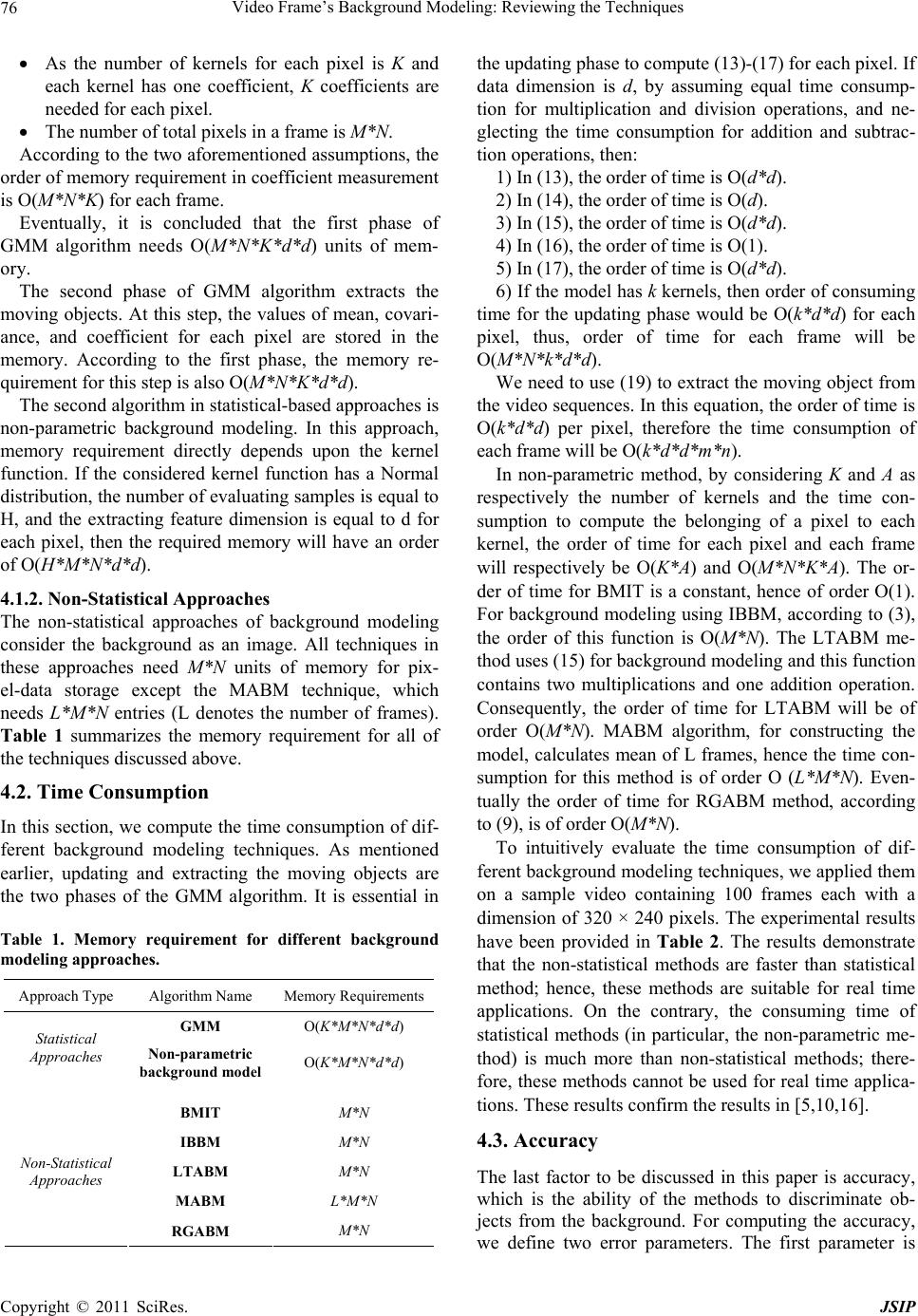

Video Frame’s Background Modeling: Reviewing the Techniques 76
 As the number of kernels for each pixel is K and
each kernel
the updating phase to c (13)-(17) for each pixel. If
data dimension is d, ing equal tinsump-
r of consuming
tim k*d*d) for each
pi
racy,
ity of the methods to discriminate ob-
has one coefficient, K coefficients are
t in coefficient measurement
and coefficient for each pixel are stored in the
m
e kernel
fu
und as an image. All techniques in
of memory for pix-
ime consumption of dif-
techniques. As mentioned
ting the moving objects are
needed for each pixel.
 The number of total pixels in a frame is M*N.
According to the two aforementioned assumptions, the
order of memory requiremen
is O(M*N*K) for each frame.
Eventually, it is concluded that the first phase of
GMM algorithm needs O(M*N*K*d*d) units of mem-
ory.
The second phase of GMM algorithm extracts the
moving objects. At this step, the values of mean, covari-
ance,
emory. According to the first phase, the memory re-
quirement for this step is also O(M*N*K*d*d).
The second algorithm in statistical-based approaches is
non-parametric background modeling. In this approach,
memory requirement directly depends upon th
nction. If the considered kernel function has a Normal
distribution, the number of evaluating samples is equal to
H, and the extracting feature dimension is equal to d for
each pixel, then the required memory will have an order
of O(H*M*N*d*d).
4.1.2. N on-Statistical Appro ach es
The non-statistical approaches of background modeling
consider the backgro
these approaches need M*N units
el-data storage except the MABM technique, which
needs L*M* N entries (L denotes the number of frames).
Table 1 summarizes the memory requirement for all of
the techniques discussed above.
4.2. Time Consumption
In this section, we compute the t
ferent background modeling
earlier, updating and extrac
the two phases of the GMM algorithm. It is essential in
Table 1. Memory requirement for different background
modeling approaches.
Approach Type Algorithm Name Memory Requirements
GMM O(K*M*N*d*d)
Statistical
Approaches Non-parametric
ackground model b
M*N
LTABM
L*M*N
O(K*M*N*d*d)
BMIT
IBBM M*N
M*N
MABM
Non-Statistical
Approaches
RGABM M*N
ompute
by assumme co
tion for multiplication and division operations, and ne-
glecting the time consumption for addition and subtrac-
tion operations, then:
1) In (13), the order of time is O(d*d).
2) In (14), the order of time is O(d).
3) In (15), the order of time is O(d*d).
4) In (16), the order of time is O(1).
5) In (17), the order of time is O(d*d).
6) If the model has k kernels, then orde
e for the updating phase would be O(
xel, thus, order of time for each frame will be
O(M*N*k*d*d).
We need to use (19) to extract the moving object from
the video sequences. In this equation, the order of time is
O(k*d*d) per pixel, therefore the time consumption of
each frame will be O(k*d*d*m*n ).
In non-parametric method, by considering K and A as
respectively the number of kernels and the time con-
sumption to compute the belonging of a pixel to each
kernel, the order of time for each pixel and each frame
will respectively be O(K* A) and O(M*N* K* A). The or-
der of time for BMIT is a constant, hence of order O(1).
For background modeling using IBBM, according to (3),
the order of this function is O(M*N). The LTABM me-
thod uses (15) for background modeling and this function
contains two multiplications and one addition operation.
Consequently, the order of time for LTABM will be of
order O(M*N). MABM algorithm, for constructing the
model, calculates mean of L frames, hence the time con-
sumption for this method is of order O (L*M*N). Even-
tually the order of time for RGABM method, according
to (9), is of order O(M*N).
To intuitively evaluate the time consumption of dif-
ferent background modeling techniques, we applied them
on a sample video containing 100 frames each with a
dimension of 320 × 240 pixels. The experimental results
have been provided in Table 2. The results demonstrate
that the non-statistical methods are faster than statistical
method; hence, these methods are suitable for real time
applications. On the contrary, the consuming time of
statistical methods (in particular, the non-parametric me-
thod) is much more than non-statistical methods; there-
fore, these methods cannot be used for real time applica-
tions. These results confirm the results in [5,10,16].
4.3. Accuracy
The last factor to be discussed in this paper is accu
which is the abil
jects from the background. For computing the accuracy,
we define two error parameters. The first parameter is

Video Frame’s Background Modeling: Reviewing the Techniques 77
Table 2. Time consumption of different techniques in mod-
eling the background of a sample video containing 100
frames each with a dimension of 320 × 240 pixels.
Algorithm Type Algorithm Name Consuming
Time Order
GMM 241.773229 s O(M*N*d*d)
Statistical
O(M*N*H*A)
LTABM O
O
Non-statistical
approach
approach Non-Parametric 981.430302
BMIT 9.817173 s O(1)
IBBM 10.200367 s O(M*N)
10.253446 s (M*N)
MABM 14.497409 s (L*M*N)
RGABM 10.151088 s O(M*N)
false negative (FN), t
sified as backgrounum
ixels. The second parameter is false positive (FP),
the approaches in
m
ound modeling techniques for indoor applications.
he number of object pixels misclas-
nd pixels over the total ber of ob-
ject p
the number of background pixels misestimated as object
pixels over the total number of background pixels. Noise
or illumination changes are the causes of FP error.
We have used four frames from two video sequences,
one indoor and one outdoor, to evaluate accuracy of each
method. The error rate parameters for the indoor video
sequence are shown in Table 3. The FN results demon-
strate that the lowest error rate belongs to MABM me-
thod; and the accuracy of GMM, LTABM, and RGAM
methods are not acceptable. The high FN error rates ex-
press that parts of the objects are not extracted success-
fully, thus, extracted objects cannot be used for object
indexing applications. The FP error rates demonstrate
that the best result belongs to GMM and RGABM me-
thod, confirming that these methods are relatively safe
against noisy conditions. The results from Table 3 indi-
cate that BMIT, IBBM, and MABM are more suitable for
indoor background modeling compared to the other ap-
proaches evaluated in this research.
Table 4 represents accuracy of
Table 3. Comparing accuracy of different backgr
odeling background of the outdoor video. The FN error
rates of BMIT, IBBM and MABM methods are very high;
therefore, the extracted objects using these approaches
are incomplete. Consequently, these methods may not be
suitable for real-world applications, which require com-
pletely identified objects. The results in Table 4 indicate
that the FN error rate in GMM and RGABM are less than
1%, however these methods have a high FP error rate.
The results indicate that any of the evaluated approaches
Frames
Frame 1 Frame 2 Frame 3 Frame 4 rage Ave
Methods
FN FN FN FN FN FP FPFP FP FP
GMM 0. 7 0. 0. 0. 0. 0. 0. 0 0 0003 0 011375480242 7337 02423721 .0150
BMIT 0 0.0080 0 0.0253 0.1418 0.0739 0.2095 0.0684 0.0878 0.0439
IBBM 0 0.0077 0 0.0089 0.1442 0.0412 0.2267 0.0363 0.0927 0.0235
LTABM 0.
0.
0 00006 0 0.0295 0.6962 0.0267 0.8754 0.0434 0.3929 0.0249
MABM 0 0.0041 0 0.0194 0.1291 0.0615 0.2135 0.0781 0.0856 0.0407
RGABM 0 00023 0 0 0.7772 0.0183 0.8690 0.0123 0.4115 0.0077
Table. Comccuraof differe backgmodchnr ouppl. 4paring acy ntround eling teiques fotdoor aications
Frames
Frame 1 Frame 2 Frame 3 Frame 4 age Aver
Methods
FN FP FNP FNFN FP F FP FN FP
GMM 0. 0. 0. 0. 0. 0. 0. 0. 0
0079 9748 0104 7911 0068 9416 00390 0073 .6769
BMIT 0.1982 0.1275 0.2316 0.0950 0.2436 0.0664 0.1707 0 0.2110 0.0722
IBBM 0.1565 0.1619 0.1752 0.0984 0.1874 0.0701 0.1392 0 0.1646 0.0826
LTABM 0.0174 0.5693 0.0397 0.5921 0.0272 0.6922 0.0187 0 0.0258 0.4634
MABM 0.1422 0.1551 0.2133 0.1040 0.1860 0.1860 0.1248 0.1248
RGABM 0.0066 0.8187 0.0121 0.7225 0.0122 0.8265 0.0073 0 0.0096 0.5919
0.1666 0.1425

Current Distortion Evaluation in Traction 4Q Constant Switching Frequency Converters 78
hr a hi or FPisved
tharamato erly for
u icat
ling methods can be classified into
atistical and non-statistical approaches.
irst group use statistical concep
. R. Wren, A. Azarbayejani, T. Darrell and A. P. Pent-
land, “Pfinderthe Human Body,”
IEEE Transacis and Machine
as eithegh FN a high, which concei
at their p
tdoor appl
meters
ions.
y need be prop tuned
o
5. Conclusions
The background mode
two main groups: st
Approaches in the fts for
background modeling. Memory requirement and con-
suming time of these methods are very high; hence, sta-
tistical approaches are not suitable for real time applica-
tions. On the other hand, these methods can be suitable
for outdoor environment if their parameters be properly
tuned, because of their safe operation in noise and sud-
den change condition. However, non-statistical methods
are very easy to implement, and memory requirement of
these approaches is very low compared to statistical me-
thods. In addition, time consumption of non-statistical
methods is rather low; consequently, these methods are
suitable for indoor environments and real-time applica-
tions.
REFERENCES
[1] C
: Real-Time Tracking of
tions on Pattern AnalysIn-
telligence, Vol. 19, No. 7, 1997, pp. 780-785.
doi:10.1109/34.598236
[2] C. Stauffer and W. E. L. Grimson, “Adaptive Background
Mixture Models for Real-Time Tracking,” IE
puter Society ConferencEE Com- e on Computer Vision and Pat-
tern Recognition, Vol. 2, No. 23-25, 1999, pp. 246-252.
[3] L. Hanzo, P. J. Cherriman and J. Streit, “Video Compres-
sion and Communications,” WILEY, 2007.
doi:10.1002/9780470519929
[4] Y. Q. Shi, H. F. Sun, “Image and Video Compression for
Multimedia Engineering,” CRC Press, Boca Raton, 2008.
doi:10.1201/9781420007268
[5] P. Kumar, K. Sengupta and A. Lee. “A Comparative
Study of Different Color Spaces for Foreground and
Shadow Detection for Traffic Monitoring System,” Pro-
4.
] P. Blauensteiner, H. Wildenauer, A. Hanbur.
KamOn Cpr Changte
Shadow Suppression,” Proceedings 1th er
st Symposium on Applied perception in
E ICCV’99
gs of the 12th
ter Society
and Machine In-
ceedings of the IEEE 5th International Conference on In-
telligent Transportation Systems, 2002, pp. 100-105.
[6] N. Schofield and C. McFarlane, “Segmentation and Track-
ing of Piglets in Images,” Machine Vision and Applica-
tions, 1995, pp. 187-193.
[7] Cavallaro, A. Salvador and E. Ebrahimi, “Detecting Sha-
dows in Image Sequences,” Visual Media Production
(CVMP), 2004, pp. 165-17
[8 y and M
ction andpel, “olour Saces foe De
of the 1Comput
Winter Vision Workshop (CVWWS6), 6-8 February 2006,
pp. 117-123.
[9] Erum A. Khan and E. Reinhard, “A Survey of Color
Spaces for Shadow Identification,” APGV ’04: Proceed-
ings of the 1
graphics and visualization, New York, 2004, p.160.
[10] M. Piccardi, “Background Subtraction Techniques: A
Review,” IEEE International Conference on Systems,
Man and Cybernetics, Vol. 4, 2004, pp. 3099-3104.
[11] A. M. Elgammal, D. Harwood and L. S. Davis, “Non-
Parametric Model for Background Subtraction,” Pro-
ceedings of ECCV 2000, 2000, pp. 751-767.
[12] T. Horprasert, D. Harwood and L. S. Davis. “A Statistical
Approach for Real-Time Robust Background Subtraction
and Shadow Detection,” Proceedings of IEE
FRAME-RATE Workshop, 1999, pp. 1-19.
[13] D. Koller, J. Weber, T. Huang, J. Malik, G. Ogasawara, B.
Rao and S. Russell, “Towards Robust Automatic Traffic
Scene Analysis in Real-Time,” Proceedin
IAPR International Conference on Computer Vision &
Image Processing, Vol. 1, 1994, pp. 126-131.
[14] N. Martel-Brisson and A. Zaccarin, “Moving Cast Shadow
Detection from a Gaussian Mixture Shadow Model,” In
CVPR ’05: Proceedings of the IEEE Compu
Conference on Computer Vision and Pattern Recognition
(CVPR’05), Vol. 2, 2005, pp. 643-648.
[15] A. Prati, I. Mikic, M. M. Trivedi and R. Cucchiara, “De-
tecting Moving Shadows: Algorithms and Evaluation,”
IEEE Transactions on Pattern Analysis
telligence, Vol. 25, No. 7, 2003, pp. 918-923.
doi:10.1109/TPAMI.2003.1206520
[16] S.-T. Su and Y.-Y. Chen, “Moving Object Segmentation
Using Improved Running Gaussian Average B
Model,” Digital Image Computing:
ackground
Techniques and Ap-
Vision Systems, Springer,
edman and S. Russell, “Image Segmentation in
ersity in Artificial In-
plications, 2006, pp. 24-30.
[17] N. Oliver, B. Rosario and A. Pentland, “A Bayesian Com-
puter Vision System for Modeling Human Interactions,”
International Conference on
1999.
[18] R. Jain, R. Kasturi and B. G. Schunk, “Machine Vision,”
McGraw-Hill Inc., 2003, pp. 63-69.
[19] N. Fri
Video Sequences: A Probabilistic Approach,” Proceed-
ings of the 13th Conference on Univ
telligence (UAI), 1997.
[20] L. Wendy and A. R. Martinez, “Computational Statistics
Handbook with Matlab,” CRC Press, 2002.