Technology and Investment
Vol.1 No.4(2010), Article ID:3212,9 pages DOI:10.4236/ti.2010.14032
An Application of Fuzzy Set Theory to the Weighted Average Cost of Capital and Capital Structure Decision
1Department of Finance, National Dong Hwa University, Shoufeng, Taiwan, China
2Department of Health Business Administration, Tajen University, Pingtung, Taiwan, China
E-mail: gracew@mail.ndhu.edu.tw, david17hwang@gmail.com
Received August 31, 2010; revised October 9, 2010; accepted October 13, 2010
Keywords: WACC, capital structure, fuzzy numbers, capital structure, fuzzy logic
Abstract
The purpose of this paper is to present the use of fuzzy logic to improve the calculation of weighted average cost of capital (WACC). The fuzzy WACC approach not only allows the pre-tax cost of debt, the effective tax rate, the tax benefit, and cost of equity to be treated as fuzzy numbers, it also offers ranking means to find the optimal debt ratio. This paper contributes to the literature by offering alternative methods to calculate the WACC and the optimal debt ratio for firms under uncertainty. Compared with the traditional WACC, the fuzzy WACC model can overcome the problems pertinent to uncertainty, complexity and imprecision. This paper thus sheds light on capital structure decision making.
1. Introduction
Sharpe [1] and Lintner [2] brought the theory of the capital asset pricing model (CAPM), which offers a very intuitive and straightforward method to gauge the cost of equity. Four decades later, the CAPM still remains the predominant model to estimate the cost of equity as shown in numerous surveys of corporate practice (Bruner et al. [3]; Bierman [4]; Gitman and Vandenberg [5]; Graham and Harvey [6]; Arnold and Hatzopoulos [7]; McLaney, Pointon, Thomas and Tucker [8]; and Brounen, De Jong and Koedijk [9]); however, a series of influential papers, based on the failure of the CAPM in empirical tests, have doubted the performance of CAPM (Chopra, Lakonishok and Ritter [10]; Fama and French [11]; Davis [12]; Barber and Lyon [13]; and Roll [14]), and argued that beta is not favorable in explaining the crosssection of stock returns. In response, several studies (Black [15]; Kothari et al. [16]; and Sharpe [17]) persisted that the CAPM is still the best model for estimating the cost of equity and all the empirical results conflicting with the CAPM are due to selection bias or the mis-measurement of beta. As the ongoing debate among researchers continues, the WACC remains a hot topic in the finance literature. Generally, multifactor models are regarded as alternatives to the CAPM for estimating the cost of equity.
The aforementioned studies have stimulated the development of asset pricing models, but both CAPM and multifactor models offer practitioners only a single rate cost of equity, which is always uncertain because the cost of equity varies over time or with market conditions in the real world, and its considerable ambiguity may mislead us to one set of optimal debt ratio calculations. So Lister [18] advocates management should cease their expensive search for the cost of equity. Furthermore, much of the evidence also implies that the cost of debt is uncertain. For example, Lund [19] has pointed out that much of the literature on the relationship between the cost of debt and taxation neglects uncertainty. Mayer [20] uses a dynamic programming model to examine the cost of debt, indicating that the current taxable earnings of the firm are highly volatile and uncertain, Graham and Harvey [6] demonstrates that the effective tax rate varies with non-debt tax shields, such as depreciation, investment tax, carry-forwards of past operating losses, and the like.
Owing to uncertainty with respect to the cost of capital, we argue that a reasonable range of the cost of capital estimates is indispensable, and then we use it in the optimal debt ratio calculations. Bruner et al. [3] conclude that best-practice companies may not give a precise number about WACC but can estimate them with an accuracy of no more than plus or minus 100 to 150 basis points. In other words, the ranges of estimated WACC are consistent with a real world, and it embeds fuzzy characteristics. In such scenario, fuzzy set theory may help mitigate uncertainty, and to our best knowledge, there is no literature applying a fuzzy set theory to the WACC and capital structure.
In addition, traditional WACC employs the marginal tax rate and assumes a constant operating income as the debt ratio increases. In our model, we modify the tax rate to reflect the potential loss of the tax benefits of debt at higher debt ratios, where the interest expenses exceed the EBIT. The effective corporate tax rate can differ from the statutory corporate tax rate because taxable income can differ from economic income due to features of the tax system, such as accelerated depreciation, industryspecific concessions or non-compliance. As a result, the effective corporate tax rate can reflect the uncertainty of future cash flows and produce meaningful estimates of tax shield and cost of debt. For this reason, we adopt the effective tax rate rather than the marginal or statutory tax rate.
In this paper we present the use of fuzzy logic as a post-processing method to improve the calculation of the WACC. The purpose of this paper is to develop fuzzy weighted average cost of capital and fuzzy capital structure with firm value maximization in mind. The fuzzy WACC approach not only allows the pre-tax cost of debt, the effective tax rate, the tax benefit, and the cost of equity to be expressed as fuzzy numbers, but also offers ranking means to find the optimal debt ratio. These fuzzy numbers can better capture the uncertainty in the computation of the WACC. Finally, In order to rank the WACC at each level of debt for seeking a precise optimal capital structure, this paper adopts the latest method for ranking generalized trapezoidal fuzzy numbers by Chen et al. [21], which we will discuss in more details later in Subsection 2.4. Our results are consistent with the trade-off theory. Compared with the traditional WACC, the fuzzy WACC model overcomes issues regarding uncertainty, complexity, and imprecision. The rest of this paper is organized as follows: Section 2 introduces the fuzzy WACC model and the latest method for ranking generalized trapezoidal fuzzy numbers. Section 3 gives a numerical example to calculate the cost of capital using fuzzy WACC model and the optimal debt ratio. Conclusions are presented in Section 4.
2. The Fuzzy Weighted Average Cost of Capital Approach
2.1. Fuzzy Numbers
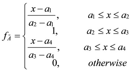
Cheng and Mon [22] describe fuzzy number A as a fuzzy subset in support R (real number), which is both normal and convex, where supp( ) = {x
  R
R  }. Normality implies that the maximum value of the fuzzy set
  in R is 1. By contrast, the maximum value of non-normal fuzzy set in R is less than 1. The concept of generalized trapezoidal fuzzy numbers attempts to deal with real problems by possibility. For a trapezoidal fuzzy number
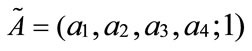 with the membership function, its membership function
 is given by
2.2. Generalized Trapezoidal Fuzzy Numbers
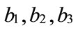
According to the characteristics of generalized trapezoidal fuzzy numbers and their operations, Figure 1 shows two different generalized trapezoidal fuzzy numbers 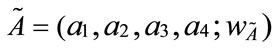 and
and , where 0 <
 ≤ 1 and 0 <
 ≤ 1;
≤ 1;  and
and  denote the degree of confidence with respect to the decision-maker's opinions A and B, respectively. We present generalized trapezoidal fuzzy numbers arithmetical operations based on the extension principle. Let
  and
and  be two generalized trapezoidal fuzzy numbers, where
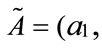
 and
and . The generalized trapezoidal fuzzy numbers arithmetic operations are as follows:
1) Generalized trapezoidal fuzzy numbers addition :
:
2) Generalized trapezoidal fuzzy numbers subtraction :
:
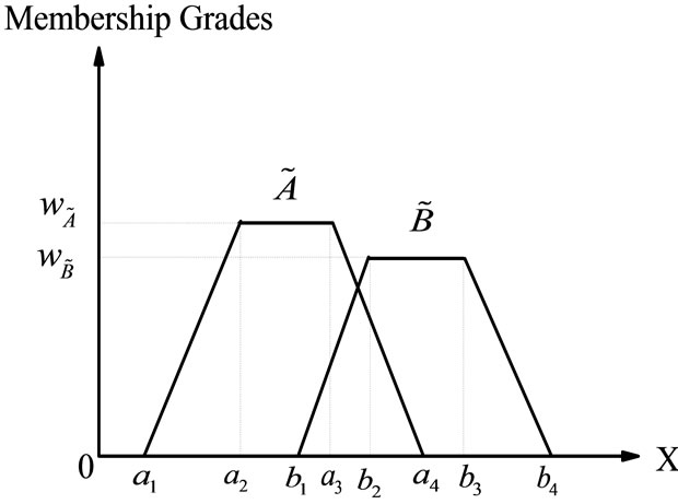
Figure 1. Generalized trapezoidal fuzzy number numbers  and
and .
.
3) Generalized trapezoidal fuzzy numbers multiplication :
:
4) Generalized trapezoidal fuzzy numbers division :
:
 .
.
where 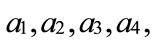
 and
and  are any real numbers.
2.3. A Fuzzy WACC Model
In this section, we use the theory of fuzzy logic to explain the WACC and capital structure decisions. When a company raises one additional dollar capital during a given time period, the costs of debt, preferred stock, and common equity begin to rise. As this happens, the marginal cost of capital (MCC) will vary according to the type of capital used. Thus, corporations cannot raise unlimited amounts of capital at a fixed cost. At some break point, the cost of each new dollar will become greater. Figure 2 graphs the marginal cost of capital (MCC) schedule as well as the retained earnings break point. Each dollar has a weighted average cost of 9 percent until the company has raised a total of $256 million. However, if firm raises more than $256 million, the WACC jumps from 9 percent to 9.5 percent. This numerical example illustrates only the concept of the increasing step function of the WACC given alternative sources of capital. The value used in each step of the WACC is by no means deterministic. In fact, WACC embeds fuzzy characteristics. This is because the decision of choosing capital structure and employing various sources of capital is fuzzy in nature. Therefore, we relate the WACC to the fuzzy logic theory and transform WACC to the fuzzy cost of capital. This can be explained in Figure 3, where fuzzy spaces exist in the triangle between b1 and a4, and between c1 and b4. These fuzzy spaces can be influenced by factors such as interest rates, exchange rates, the firm’s bargaining ability, collateral, etc.
In general, these inputs cannot be characterized by a single number. But practitioners are able to estimate the WACC by using trapezoidal possibility distribution of the form

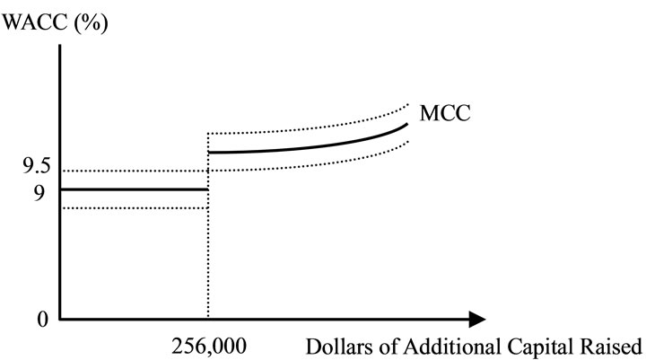
Figure 2. Marginal cost of capital schedule with the retained earnings break point.
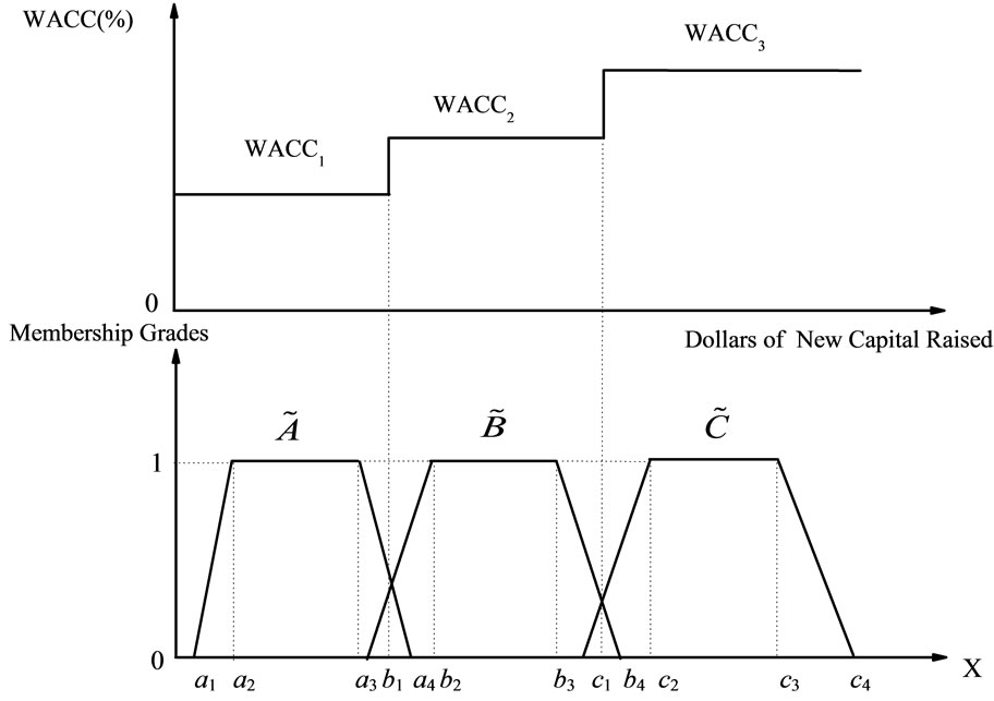
Figure 3. Combining the WACC with generalized trapezoidal fuzzy numbers.
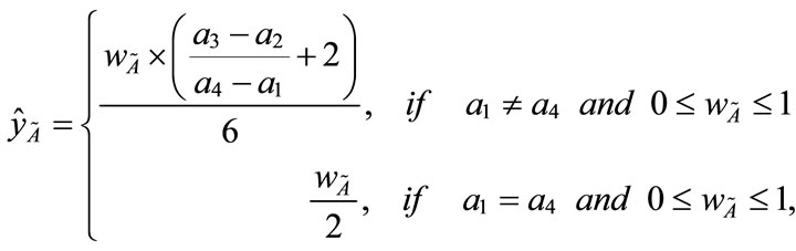
That is, the most likely values of the WACC lie in the interval between  and
and  which are the core of the trapezoidal fuzzy number
 ; while
  is the greatest value and
  is the smallest value for the WACC.
Accordingly, one can estimate the pre-tax cost of debt by using a trapezoidal possibility distribution of the form: , i.e. the most possible values of the pre-tax cost of debt lie in the interval between
  and
and  which are the core of the trapezoidal fuzzy number
 ;
;  is the greatest value and
  is the smallest value for the pre-tax cost of debt .
As we have discussed earlier, we examine the approach for estimating the costs of debt, equity, and the appropriate weights to use in computing the cost of capital. To summarize, the cost of equity should reflect the risk of an equity investment and the cost of debt should reflect the default risk of the firm. The cost of debt should also reflect the effective tax rate, and the tax benefit associated with debt. Hence, we estimate these inputs by a trapezoidal possibility distribution of the form:

i.e., the most likely values of the cost of equity, the effective tax rate, and the tax benefit lie in the interval between  and
and ,
,  and
and ,
,  and
and , respectively (which are the core of the trapezoidal fuzzy number
 ,
,  , and
, and ).
).  is the greatest value and
 is the smallest value for the cost of equity;
  is the greatest value and
  is the smallest value for the effective tax rate;
 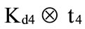 is the greatest value and
 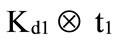 is the smallest value for the tax benefit.
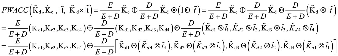
The information needed for the WACC is generally not known with certainty. The sources of uncertainty may be the pre-tax cost of debt, the cost of equity, the effective tax rate, the tax benefit, and the discount rate, etc. Under these circumstances we suggest the use of the following formula for computing the fuzzy WACC.
2.4. The Latest Ranking Method for Generalized Trapezoidal Fuzzy Numbers
From Cheng [23] and Chu [24], we can see that some methods have been proposed for ranking fuzzy numbers. Drawbacks exist in the existing ranking methods, i.e. they cannot correctly rank fuzzy numbers in some situations. Thus, in this paper, we adopt the latest method for ranking generalized trapezoidal fuzzy numbers. The latest method by Chen et al. [21] not only considers the centroid points, but also the standard deviations of generalized trapezoidal fuzzy numbers to deal with the fuzzy-number ranking problems.
Furthermore, the latest method also can rank more than two fuzzy numbers simultaneously. This method contains five steps described as follows:
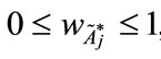
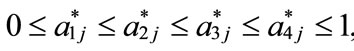
Step 1: Standardized generalized trapezoidal fuzzy numbers Assume that there are n generalized trapezoidal fuzzy number  where
where 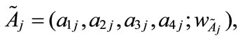 1 ≤ j ≤ n,
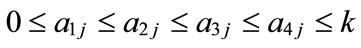
 , and k is any real value; the value
  denotes the maximum membership value of the generalized trapezoidal fuzzy number
 , where 1 ≤ j ≤ n. For each generalized trapezoidal fuzzy number
 , where 1 ≤ j ≤ n, if the generalized trapezoidal fuzzy number
  is not a standardized generalized trapezoidal fuzzy number, where the universe of discourse of the generalized trapezoidal fuzzy number
  is [0, k], then the generalized trapezoidal fuzzy number
  can be translated into a standardized generalized trapezoidal fuzzy number
  shown as follows:
 (2)
(2)
where 
 or
or , and 1 ≤ j ≤ n.
Step 2: Calculating the centroid point ( ,
, ) of each standardized generalized trapezoidal fuzzy number
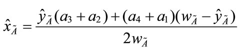 (3)
(3)
 (4)
(4)
 (1)
(1)
Step 3: Calculating the standard deviation,  of each standardized generalized trapezoidal fuzzy number
  as follows:
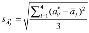 (5)
(5)
Step 4: Using the standard deviation and the value of the centroid point (
 ,
, ),
), , to derive a new value
  shown as follows:
 (6)
(6)
Step 5: Using the new point to calculate the ranking value score of the standardized generalized trapezoidal fuzzy numbers
 , where 1 ≤ j ≤ n as follows:
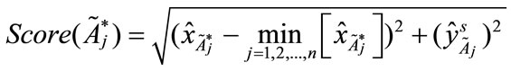 (7)
(7)
3. Example
3.1. Fuzzy WACC
In this section, we present an example to calculate the cost of capital for Boeing using fuzzy weighted average cost of capital model, where the cost of equity, the cost of debt, the tax benefit, the effective tax rate, and the weighted average cost of capital are estimated by trapezoidal fuzzy numbers.
The inputs needed to estimate the WACC can be obtained from the annual report or other sources such as the COMPUSTAT database. We analyze the optimal capital structure for Boeing in 1999 using data from Damodaran [25]. Table 1 is drawn from Damodaran, who calculated the cost of capital at each level of debt for Boeing. Table 1 provides three basic inputs to compute the cost of capital-the cost of equity, the cost of debt, and the weights on debt and equity. In addition, it estimates Boeing’s dollar amount of debt and interest expenses at each debt ratio, computes the interest coverage ratio that measures default risk to estimate a rating for Boeing, and then finds the rating that corresponds to that level of debt. According to Damodaran’s approach, the interest expense is measured by circular reasoning. This process is reiterated for each level of debt from 10% to 90%, and the pre-tax costs of debt are achieved at each level of debt.
Now let’s examine this computation in more details in Table 1. First, it presumes the EBIT at Boeing to be unaffected by the firm’s financing decision. Second, it reflects the possible losses of the tax shields of debt at higher debt ratios by modifying the effective tax rate. To explain this point, it is important to note that the EBIT at Boeing is $1,751 million. Under the condition that interest expenses are less than $1,751 million, interest expenses are fully tax deductible and earn the 35% tax benefit. For example, at a 30% debt ratio, the interest expenses are $857 million, and the tax shield is therefore 35% of this amount, and the effective tax rate is 35%. At a 60% debt ratio, however, the interest expenses rise to $2,692 million, which is greater than the EBIT of $1,751 million. At most the tax benefit on the interest expenses is $612.85 million ($1,751 million × 0.35). As the proportion of the tax benefit on the interest expenses to the total interest expenses is $612.85 million/$2,692 million, the effective tax rate is 27.76% instead of 35% on taxable income. As a matter of fact, the effective tax rate is typically a more accurate reflection of a company's tax liability than its marginal tax rate.
Based on the above-mentioned statements, the effective tax rates are unchanged and certain at the level of debt from 10% to 40%. That is, interest expenses remain fully tax deductible and earn the 35% tax benefit. But the effective tax rates are uncertain at the level of debt from 50% to 90%. Hence, only the effective tax rates at the level of debt from 50% to 90% are estimated by trapezoidal fuzzy numbers shown in Table 2.
Lund [19] has pointed out that much of the literature on the relationship between the cost of debt and taxation neglects uncertainty because the tax system is fiendishly complicated. Given its uncertainty and complexity, in Table 2 we begin the illustration by computing fuzzy pre-tax cost of debt, fuzzy effective tax rate, and fuzzy tax benefit at each debt level using trapezoidal fuzzy numbers. As firms borrow more, their default risk will increase and so will the pre-tax cost of debt (Columns 1 and 2). On the other hand, the tax benefits from debt increase as the effective tax rate goes up (Columns 3 and 4).
According to a fuzzy WACC model in Subsection 2.3, we may compute fuzzy after-tax cost of debt, fuzzy cost of equity, and fuzzy WACC at each level of debt in Table 3 using fuzzy pre-tax cost of debt, fuzzy effective tax rate, and fuzzy tax benefits obtained from Table 2 and Equation (1).
For instance, at a 50% debt ratio in Table 3, fuzzy WACC (Column 4) is equal to 50% [11.18, 12.49, 13.81, 15.12] + 50% [8.5 – (11.5 × 0.35), 9.5 – (10.5 × 0.32), 10.5 – (9.5 × 0.29), 11.5 – (8.5 × 0.26)] = [7.85, 9.34, 10.80, 12.23].
3.2. Ranking Fuzzy WACC Numbers
For the purpose of calculating Boeing’s optimal debt ratio, we adopt the latest method by Chen et al. [21] for ranking generalized trapezoidal fuzzy WACC numbers in Table 4.
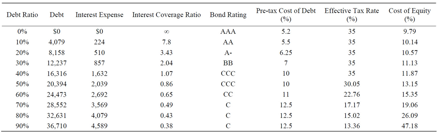
Table 1. Cost of debt, debt ratios, and cost of equity for Boeing.
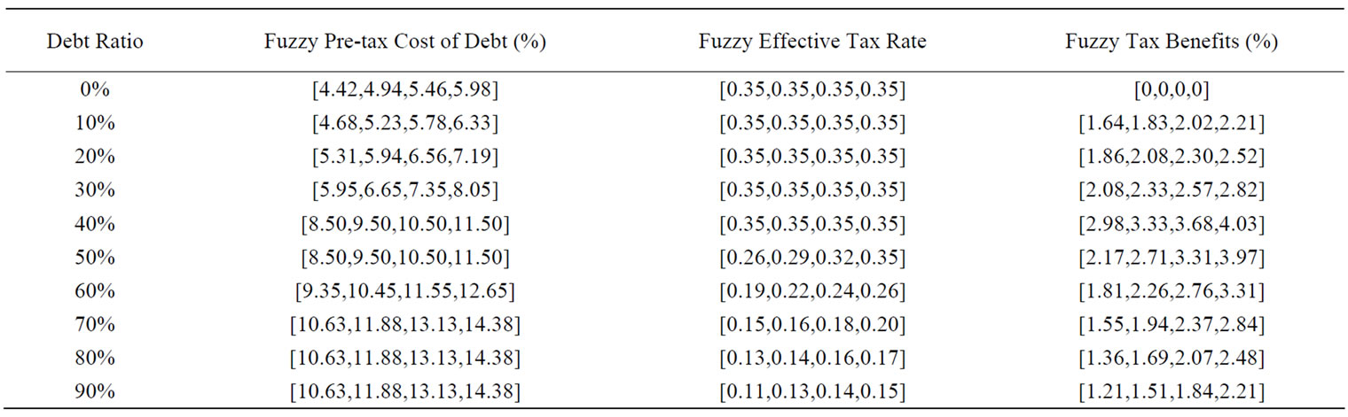
Table 2. Illustration of fuzzy pre-tax cost of debt, fuzzy effective tax rate, and fuzzy tax benefits.
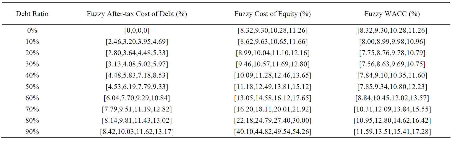
Table 3. Fuzzy after-tax cost of debt, fuzzy cost of equity and fuzzy weighted average cost of capital.
Now we rank FWACC0%, FWACC10%,…, FWACC90% shown as follow:
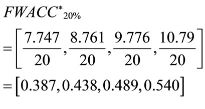
Step 1: In the process of standardizing generalized trapezoidal fuzzy WACC numbers, we have chosen 20 as the denominator since k is any real value. For example, at a 20% debt level, we translate the generalized trapezoidal fuzzy number FWACC20% = [8.003, 8.990, 9.977, 10.964] into a standardized generalized trapezoidal fuzzy number FWACC*20% shown as follows:
Step 2: Based on Equations (3) and (4), we can get the centroid point ( ,
, ) of the standardized generalized trapezoidal fuzzy number as follows: FWACC0% is [0.4895, 0.3889]; FWACC10% is [0.4742, 0.3889]; FWACC20% is [0.4634, 0.3889];… and FWACC90% is [0.7221, 0.3889].
Step 3: Based on Equation (5), we can get the standard deviation ( ) of the standardized generalized trapezoidal fuzzy number as follows: FWACC0% is 0.063194; FWACC10% is 0.063701; FWACC20% is 0.065476; … and FWACC90% is 0.12248.
Step 4: Based on Equation (6), we can get a new point  = [0.4895, 0.475424] of the standardized generalized trapezoidal fuzzy number as follows: FWACC0% is [0.4895, 0.475424]; FWACC10% is [0.4742, 0.475227]; and FWACC90% is [0.7221, 0.452369].
Step 5: Based on Equation (7), we can see that the ranking value score (FWACC0%) of the standardized generalized trapezoidal fuzzy number FWACC0% is 0.47648; the ranking value score (FWACC10%) of the standardized generalized trapezoidal fuzzy number FWACC10% is 0.475509;… and the ranking value score (FWACC90%) of the standardized generalized trapezoidal fuzzy number FWACC90% is 0.52394.
Moreover, in Table 4, the minimum ranking value score is the standardized generalized trapezoidal fuzzy number of 0.46552, which minimizes the overall cost of capital. Hence, Boeing’s optimal debt ratio is 50%. The ranking value score, which is 0.47648 when the firm is unlevered, decreases as the firm initially adds debt, reaches a minimum of 0.46552 at a 50% debt, and then starts to increase again. The optimal debt ratio for Boeing is shown graphically in Figure 5.
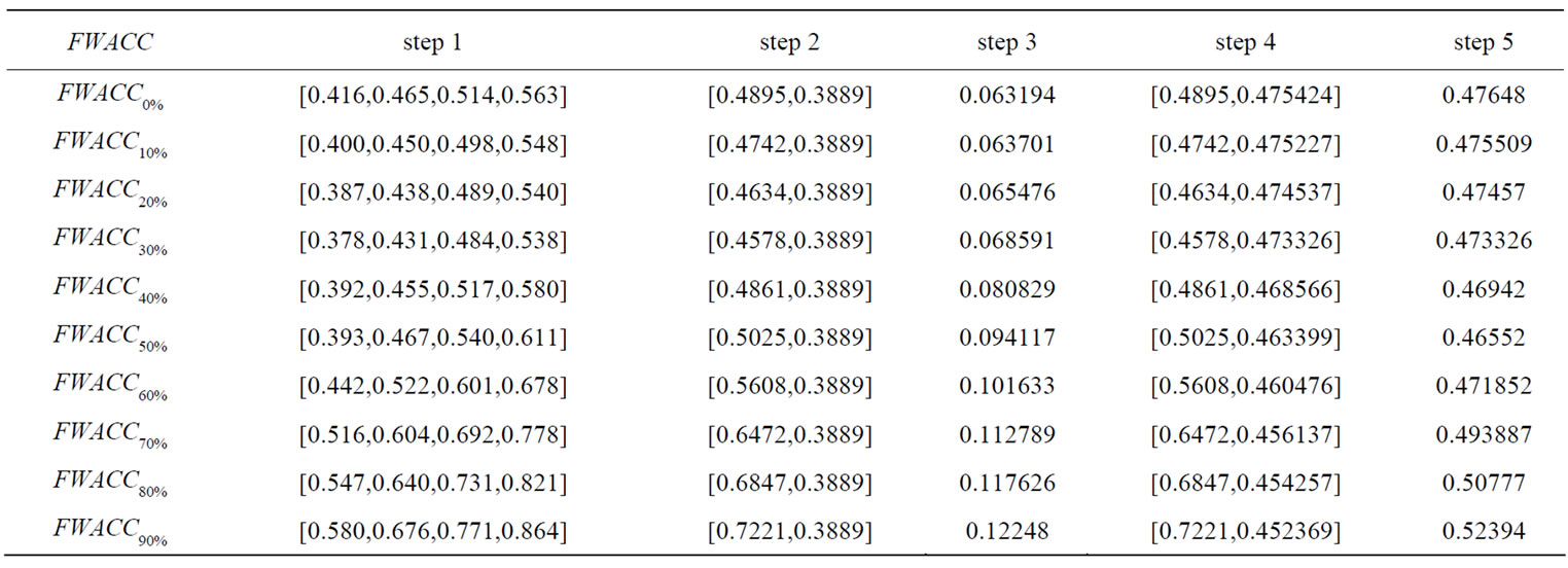
Table 4. A new ranking method for the generalized trapezoidal fuzzy numbers.
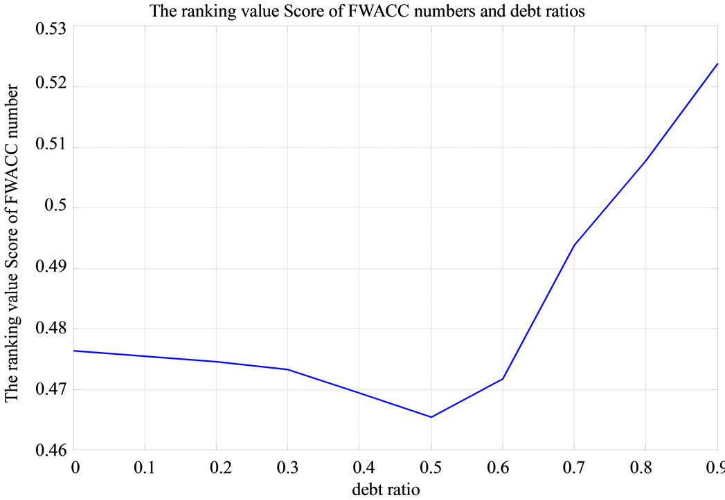
Figure 5. The ranking value score of trapezoidal fuzzy numbers and debt ratios.
Using fuzzy logic to analyze WACC and optimal capital structure, we find that WACC follows a U-shaped curve. That is, the fuzzy WACC decreases initially with the increase of debt ratio. However, the fuzzy WACC begins to increase when the debt ratio exceeds 50%. Therefore, the lowest fuzzy WACC is achieved when the debt ratio is at the 50% level. For debt ratio of 50%, it means that the WACC will lie within the closed interval [0.5025, 0.463399] with a new ranking method. From another point of view, if a practitioner is comfortable with this new ranking method, then he/she can pick up any value from the closed interval [0.5025, 0.463399] as the WACC for his/her later use.
4. Conclusions
Due to the uncertainty in the capital markets and incomplete information, decision makers often possess only fuzzy information for the decision variables. This study combines fuzzy logic theory, the concept of WACC and optimal capital structure. Such integration allows decision makers to estimate the upper and lower bounds of the cost of capital given a debt ratio, hence making optimal decisions under uncertainty with fuzzy information. In general, the traditional WACC assumes implicitly that the level of cash flows to the firm is unaffected by the firm's financing mix, which might be unreasonable in the real world. This paper sheds light on making capital structure decisions. We suggest that the fuzzy WACC model can be used as an alternative way to estimate a firm's WACC. Furthermore, the fuzzy WACC model takes explicitly the issues of uncertainty, complexity, and imprecision. The fuzzy WACC approach allows the pre-tax cost of debt, the effective tax rate, the tax benefit, and the cost of equity to be fuzzy numbers; it also offers ranking means to find the optimal debt ratio. Finally, we would like to stress that advanced decision methods such as fuzzy capital structure and fuzzy WACC open the door of opportunity to explore the optimal debt ratio for a firm, and give further insight into the real uncertainty of the cost of capital. The proposed model may give practitioners a better understanding of the problem when making the financing mix choices.
5. References
[1] W. F. Sharpe, “Capital Asset Prices,” Journal of Finance, Vol. 13, No. 3, September 1964, pp. 425-442.
[2] J. Lintner, “The Valuation of Risk Assets and the Selection of Risky Investments in Stock Portfolios and Capital Budgets,” Review of Economics and Statistics, Vol. 47, 1965, pp. 13-37.
[3] R. F. Bruner, K. M. Eades, R. S. Harris and R. C. Higgins, “Best Practices in Estimating the Cost of Capital: Survey and Synthesis,” Financial Practice and Education, Vol. 8, No. 1, 1998, pp. 13-28.
[4] H. J. Bierman, “Capital Budgeting in 1992: A Survey,” Financial Management, Vol. 22, 1993, p. 24.
[5] L. J. Gitman and P. A. Vandenberg, “Cost of Capital Techniques Used by Major US Firms: 1997 vs. 1980,” Financial Practice and Education, Vol. 10, No. 2, Fall/ Winter, 2000, pp. 53-68.
[6] J. R. Graham and C. R. Harvey, “The Theory and Practice of Corporate Finance: Evidence from the Field,” Journal of Financial Economics, Vol. 60, No. 2-3, 2001, pp. 187-244.
[7] G. Arnold and P. Hatzopoulos, “The Theory-Practice Gap in Capital Budgeting: Evidence from the United Kingdom,” Journal of Business Finance and Accounting, Vol. 27, No. 5-6, 2000, pp. 603-626.
[8] E. McLaney, J. Pointon, M. Thoma and J. Tucker, “Practitioners’ perspectives on the UK cost of capital,” European Journal of Finance, Vol. 10, No. 8, 2004, pp. 123- 138.
[9] D. Brounen, A. De Jong and K. Koedijk, “Corporate Finance in Europe: Confronting Theory with Practice,” Financial Management, Vol. 33, No. 4, 2004, pp. 71-101.
[10] N. Chopra, J. Lakonishok and J. R. Ritter, “Measuring Abnormal Performance: Do Stocks Overreact,” Journal of Financial Economics, Vol. 31, No. 2, 1992, pp. 235- 268.
[11] E. F. Fama and K. R. French, “The Cross-section of Expected Stock Returns,” The Journal of Finance, Vol. 47, No. 2, 1992, pp. 427-465.
[12] J. L. Davis, “The Cross-section of Realized Stock Returns: The PRE-COMPUSTAT Evidence,” Journal of Finance, Vol. 49, No. 5, 1994, pp. 1579-1593.
[13] B. M. Barber and J. D. Lyon, “Firm Size, Book-to-Market Ratio, and Security Returns: A Holdout Sample of Financial Firms,” Journal of Finance, Vol. 52, No. 2, 1997, pp. 875-883.
[14] R. Roll, “A Critique of the Asset Pricing Theory’s Tests,” Journal of Financial Economics, Vol. 4, No. 2, 1977, pp. 129-176.
[15] F. Black, “Beta and Return,” Journal of Portfolio Management, Vol. 20, No. 1, 1993, pp. 8-18.
[16] S. P. Kothari, J. Shanken and R. G. Sloan, “Another Look at the Cross-Section of Expected Returns,” Journal of Finance, Vol. 50, No. 1, 1995, pp. 185-224.
[17] W. F. Sharpe, “Factor Models, CAPMs and the APT,” Journal of Portfolio Management, Vol. 11, 1984, pp. 21- 25.
[18] R. Lister, “Cost of Capital is Beyond Our Search,” Accountancy, Vol. 138, No. 1360, 2006, pp. 42-43.
[19] D. Lund, “Taxation, Uncertainty, and the Cost of Equity,” International Tax and Public Finance, Vol. 9, 2002, pp. 483-503.
[20] C. Mayer, “Corporation Tax, Finance and the Cost of Capital,” Review of Economic Studies, Vol. 53, No. 1, 1986, pp. 93-112.
[21] S. J. Chen and S. M. Chen, “Fuzzy Risk Analysis Based on the Ranking of Generalized Trapezoidal Fuzzy Numbers,” Applied Intelligence, Vol. 26, No. 1, 2007, pp. 1- 11.
[22] C. H. Cheng and D. L. Mon, “Fuzzy System Reliability Analysis by Confidence Interval,” Fuzzy Sets and Systems, Vol. 56, May 1993, pp. 29-35.
[23] C. H. Cheng, “A New Approach for Ranking Fuzzy Numbers by Distance Method,” Fuzzy Sets and Systems, Vol. 95, No. 1, 1998, pp. 307-317.
[24] T. C. Chu, “Ranking Fuzzy Numbers with an Area Between the Centroid Point and Original Point,” Computers and Mathematics with Applications, Vol. 43, No. 2, 2002, pp. 111-117.
[25] A. Damodaran, “Corporate Finance: Theory and Practice,” John Wiley & Sons, New York, 2001.