Technology and Investment
Vol.1 No.3(2010), Article ID:2495,4 pages DOI:10.4236/ti.2010.13023
Evaluation of Venture Capital Based on Evaluation Model
Department of Mathematics, Wuhan University of Technology, Wuhan, China
E-mail: {tonghengqing, pych1220}@126.com
Received March 28, 2010; revised April 16, 2010; accepted April 28, 2010
Keywords: Venture Capital, Evaluation Model, Least Squares Estimation, Interactive Projection Algorithm
Abstract
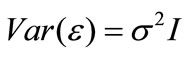
This paper studies evaluation problem in venture capital. Based on the venture capital and the actual evaluation work, we use an evaluation model proposed by us to evaluate the profitability of enterprises. We establish the impact of investment income and investment risk index system, corresponding to get observational data of the second order indexes. Evaluation model is a kind of generalized linear regression model with convex constraint, in which the dependent variable is unknown and regression coefficients all are calculated in accordance with samples instead of the prior designated. The least squares estimation of the model is given by the interactive projection algorithm between the convex sets, so as to provide a new analysis method for venture capital evaluation index system.
1. Introduction
The so-called venture capital assessment is to give an assessment of the benefits and the risk of investment projects according to the commercial prospectus based on the information collection [1]. Evaluation index system is the tool and method of the project evaluation, as a support system for investment appraisal. It links up the investment appraisal and assessment objective organically, and plays a role as a bridge and link, which is indispensable in investment appraisal.
Foreign countries have already set up comparatively perfect assessment index system of venture capital. In our country, venture capital is still a new thing, which has not set up comparatively perfect assessment index system yet, so for promoting development of venture capital in China, it is necessary to set up an assessment index system that is suitable for China’s actual conditions in venture capital.
2. Venture Capital Evaluation Index System
The assessment index system of venture capital is an indispensable tool and method in the evaluation process of the venture capital. Scientific and effective assessment index system can help the professional personnel of venture capital to assess venture projects, according to the principle of investment, risk partiality and certain assessment criterion and method. It can exclude projects whose risks are too high or profits are too low among a large number of projects, and choose the investment project that has most appreciable potentiality [2].
According to the economic characteristics, we propose the impact factors of China’s venture capital assessment and the main index system as shown in Table 1.
When we build the index system of venture capital assessment, we can get the data record of each index, and then the index should be gathered. In general, the gathering coefficients or weighted coefficients are assigned beforehand. In this paper we consider the weighted coefficients are calculated by samples but not man-made. Thus we should introduce a mathematical model for evaluation.
3. Evaluation Model
In our evaluation model there are  objects to be evaluated,
  indexes for evaluation, and
  evaluates scores for each object and each index. We need to gather the evaluation score by weighted coefficients
 but which are unknown.
 indexes are variables and noted as
 . The evaluation value in
 evaluation for
 object and by
 index is noted as
 . The evaluation value data with
  dimension for an object in an evaluation is a row in the data matrix. There are
  rows for an object and is a data block. There are
  data blocks in the data matrix
 .
.  is a cubic matrix and can be arranged as different form by the regulation of cubic matrix. In this paper we arrange
  as
as  rows with
  columns. The score of the last evaluation for each object is
 , and they are unknown also.
The evaluation model with unknown dependent variable is a generalized linear regression model. We must add some constraint for the model to solve it. Of course the weighted coefficients must satisfy
 (i.e.
(i.e. ), and
 (i.e.
(i.e. ). This is a prescription constraint. The dependent variables must also satisfy some constraints. Obviously we only give a unique score for each evaluation object. That is, we only give
  score although there
  rows in the matrix. We define dependent variable
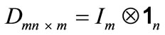
 , here
 ,
,  ,
,  ,
,  , and
, and  is Kronecker product.
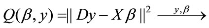
Thus the evaluation model may be expressed as following:
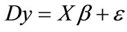 (1)
(1) ,
,
 (2)
(2)  ,
,
This model is proposed by us in [3]. The data structure of evaluation model is as the Table 2.
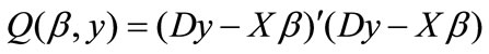
4. The Least Square Solution of the Generalized Linear Regression Model with Convex Constraint
We’ll discuss the LSE of the evaluation model in three steps [4-6].
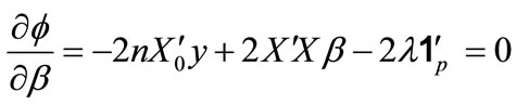
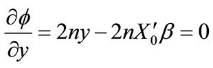
Firstly, if  is known, it is just an ordinary constraint regression model. Only considering the constraint
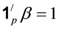 , we can get an explicit solution by the method of Lagrange Multiplier. Let
 (3)
(3)
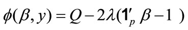 (4)
(4)
where  be the multiplier. We have
 (5)
(5)
 (6)
(6)
where
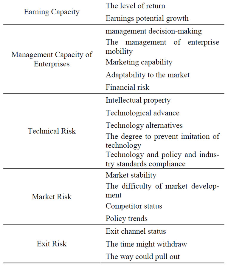
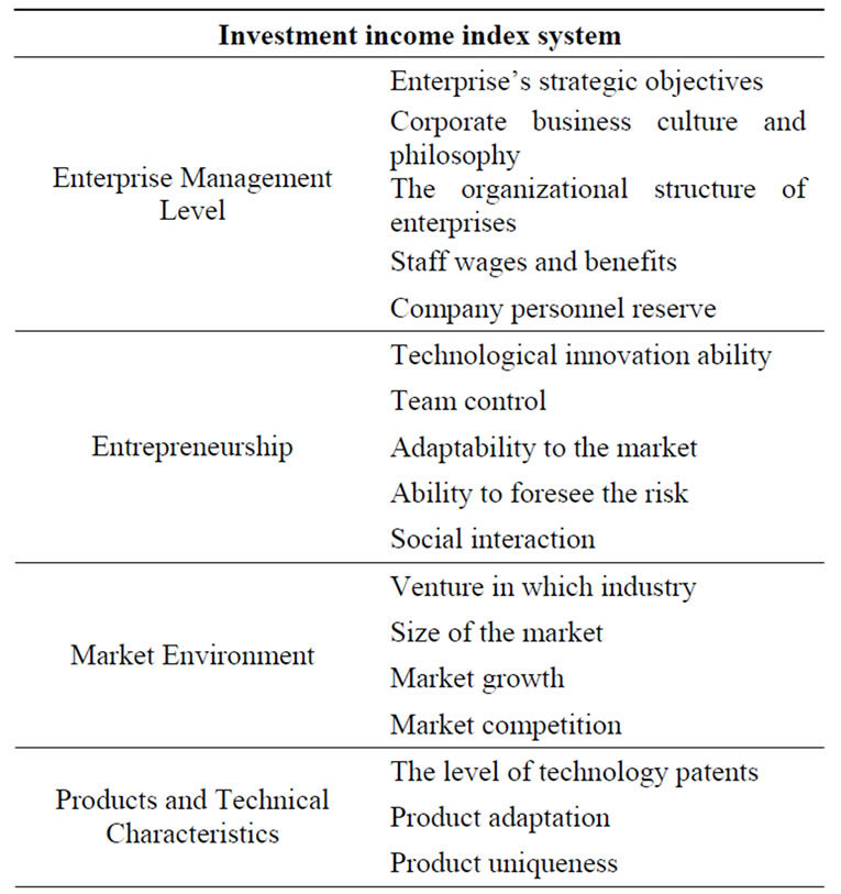
Table 1. Venture capital evaluation index system.
 (7)
(7)
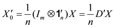
It is a compression matrix by taking the average value of each column for each data block in matrix . Then
 (8)
(8)
Let
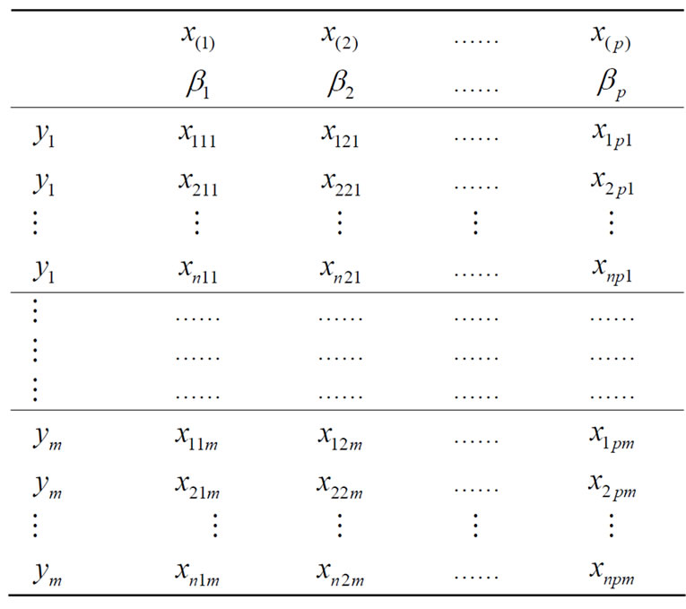
Table 2. The data structure of evaluation model.
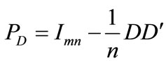 (9)
(9)
It is easy to verify that  is a projection matrix. Since
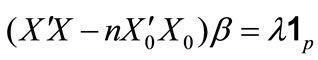 , letting
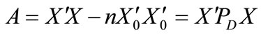 (10)
(10)
when A is invertible, the solution of  is
is
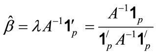 (11)
(11)
Summarizing the aforesaid, we have the following theorem.
THEOREM 1. If  is known and
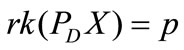 , under the constrain
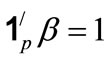 ,
,
 min(12)
has unique solution (8) and (11). If each component of  is nonnegative, (8) and (11) are also the solution of the evaluation model (1) (2).
Secondly, if some components of  are negative, we must consider the constraints
  and
and  simultaneously. Then it is a prescription regression model. For the existence and uniqueness of the solution of the model (1) (2) , we have the following theorem.
THEOREM 2. If , the evaluation model has unique solution.
The proof is easy when we rewrite (12) as
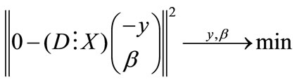 (13)
(13)
the set
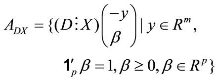 (14)
(14)
is a closed set, so there exists an unique point  and
and  satisfies (13). Because the column of
  is full rank, we can obtain unique solution of
  and
and  from
from .
.
Thirdly, we’ll discuss the algorithm of the model when  is unknown. We consider the geometric background of (12). Denote sets
 (15)
(15)
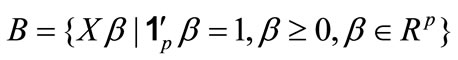 (16)
(16)
The Formula (12) means to seek the shortest Euclidean distance between sets  and
and . Obviously,
  and
and  are two closed convex sets and
  is bounded. According to the theorem “the distance between two closed convex sets can be reached”, the solution of (12) exists.
How to find the shortest distance between two convex sets? We consider the method of the alternating projection between two sets. Let  be a point in the set
 . If
. If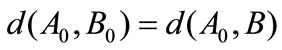 , we call
  the projection from the point
  to the set
 . The following is the alternating projection process.
Take an arbitrary initial value , find
 , satisfying
 . For
. For , take
 , satisfying
 . For
. For , take
 , satisfying
  =
= . For
. For , take
 , satisfying
 , and so on. When
 , iterative process is stopped and computation is completed. The meaning of convergence of aforesaid iterative process is:
 (17)
(17)
where  are two points which belong to sets
  and
and  respectively.
In one word, the distance between two closed convex sets may be obtained by making use of successive computation of distance between a point and a closed convex set. In the evaluation model consisting of (1) (2), for arbitrary , we can get the solution of
  according to the Theorem 1 and 2. For the solution of
 , (1) becomes a common multivariate regression model which can be solved. The convergence of the alternating projection iterative process has been proved in [3] and is omitted here.
5. Example
The following example is given by the DASC software developed by ourselves. The evaluation model data has 30 rows and 6 columns. Evaluation marks are all set from 1 to 10. The martix of evalution data is as the Table 3.
The computation process shows the convergence process is very fast and it has iterated 7 times altogether. The subprogram gives an initial value  and a control precision 0.0001. The sum of regression coefficients should be 1 in the printing result of iterative process.
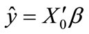
Notice that the three different fitted values of  are the evaluation results actually. And the observation value of
  is calculated according to fitting equation. The fitting effect figure provides a visual awareness of
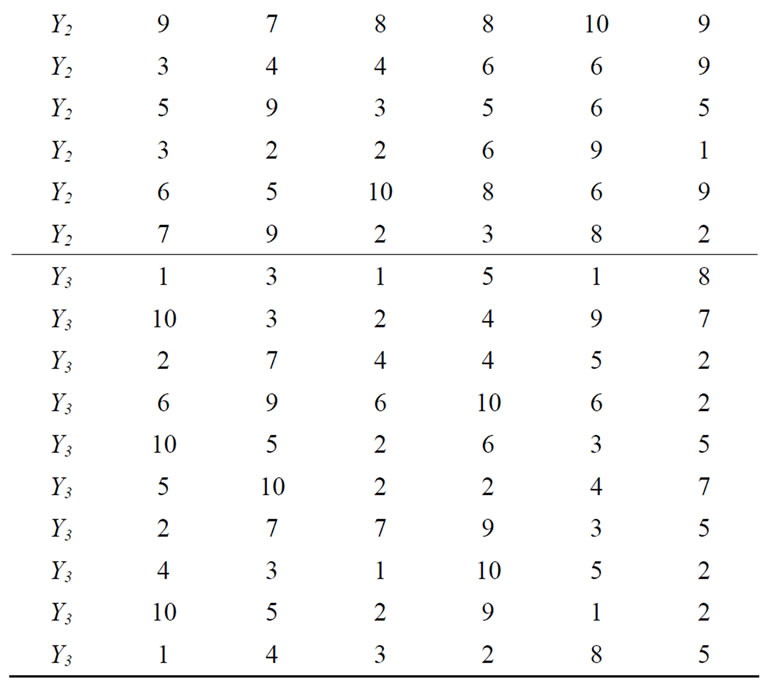
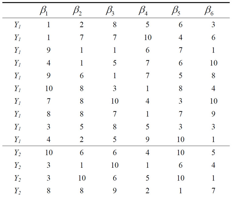
Table 3. The martix of evalution data.
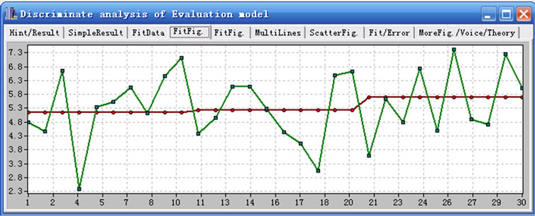
Figure 1. The fitting effect figure.
evaluation model. Results are  = 5.1451, 5.2407, 5.6958),
  = (0.2298, 0.2106, 0.1510, 0.0588, 0.2457, 0.1041), where
  is the final evaluation mark and
  is the regression coefficient, also called weight coefficient.
Evaluation model can be used as the basis for clustering. When we input X = (2, 3, 4, 5, 6, 7) in the prediction program, the forecast value is 5.1190. It denotes that this group data should attribute to the fist group, because the difference between 5.1190 and 5.1451 is the minimum.
6. Conclusions
In this paper, we studied the index system of risk evaluation for venture capital, and gave the algorithms of model in which the gathering coefficients of index were calculated by samples. Our algorithm also provides a solution scheme for some problems in venture capital evaluation, so this paper gives a new idea for venture capital evaluation with some practical reference value.
7. References
[1] Z. W. Zhao, “Research on the Appraisal and DecisionMaking in Venture Capital,” Management Science and Engineering (Professional), Tianjin University, Doctoral Dissertation, 2005.
[2] Z. H. Wang and L. Li, “Comparison of Venture Capital Assessment,” Journal of Nanhua University (Social Science Edition), Vol. 8, No. 1, February 2007, pp. 43-45.
[3] H. Q. Tong, “Evaluation Model and its Iterative Algorithm by Alternating Projection,” Mathematical and Computer Modelling, Vol. 18, No. 8, 1993, pp. 55-60.
[4] H. Q. Tong, S. J. Zhong, T. Z. Liu and Y. F. Deng, “Biostatistics Algorithm: Evaluation Model with Convex Constraint and its Parameters Estimates,” The 1st International Conference on Bioinformatics and Biomedical Engineering, 2007, pp. 402-405.
[5] H. Q. Tong, “Theory of Economics,” Science Press, 2005, pp. 262-264.
[6] K. T. Fang and S. D. He, “Regression Models with Linear Constraints and Nonnegative Regression Coefficients,” Mathematica Numerica Sinica, Vol. 7, 1985, pp. 97-102.