Journal of Electromagnetic Analysis and Applications
Vol.5 No.8(2013), Article ID:35493,6 pages DOI:10.4236/jemaa.2013.58053
Compression of Characteristics of Trajectories in Rotating Frames vs. Nonuniform Magnetic Fields
![]()
University College, The Pennsylvania State University, York, USA.
Email: has2@psu.edu
Copyright © 2013 Haiduke Sarafian. This is an open access article distributed under the Creative Commons Attribution License, which permits unrestricted use, distribution, and reproduction in any medium, provided the original work is properly cited.
Received May 11th, 2013; revised June 12th, 2013; accepted July 20th, 2013
Keywords: Rotating Frames; Coriolis Force; Inhomogeneous Magnetic Field; Mathematica
ABSTRACT
The equation of motion of an object moving in a frictionless horizontal rotating frame is somewhat comparable to the one describing the motion of a point-like charged particle projected in a magnetic field. We show the impact of angular velocity in the former is equivalent to the impact of the magnetic field in the latter. We consider scenarios conducive to comparable trajectories for these two distinct areas of physics. We extend the analysis considering two separate routes. For the rotating frame we investigate the impact of friction and for the magnetic field the effect of field in-homogeneities. We utilize Mathematica [1] throughout, most notably for solving coupled partial differential equations.
1. Introduction
Comparing the equations describing the motion of a massive object in a rotating frame vs. the ones describing the motion of a point-like charged particle in a magnetic field reveals numerous similarities. These two individual topics, the one that applies to mechanical systems and the other that applies to magneto-static field have been studied extensively but separately. A quick search of websites lists countless yet similar trivial articles concerning magneto-static cases, e.g. [2]. These references hardly address the field inhomogeneities. Classic text books such as [3] passively deal with inhomogeneities. For the rotating frames there are numerous resources as well [4,5] including the original work [6] and a classic [7]. Aside from these numerous isolated scattered resources, the author has been unsuccessful in locating an article recognizing the common features of these two separate areas of physics.
To address this issue, for the sake of simplicity we confine the analysis to two-dimensional motions. Therefore, mathematically speaking the equations describing these scenarios become a comparable paired set of coupled partial differential equations. From a physics point of view, the coefficients of the variables in one set of equations become comparable to the coefficients of variables in the other set. Merely based on this observation one anticipates the impact of varying the angular velocity on the kinematics of the former to be similar on the kinematics of the latter by varying the corresponding magnetic field. The primary objective of this article is to validate quantitatively the accuracy of this observation. Asides from the main objective, as a secondary goal, by including a symmetry breaking term such as friction we extend the analysis of the kinematics in the rotating frame. This is a fresh addition to the body of knowledge [4] now in 5th edition.
The equations describing motion with friction are nontrivial nonlinear set of paired coupled partial differential equations. These are not analytically solvable equations; neither are the equations of motion of a charged particle in an inhomogeneous magnetic field. Computer Algebra System (CAS) such as Mathematica is proven essential and noteworthy for providing numeric solutions for these equations. Needless to mention this software has been the CAS of the author’s preferred choice for the last quarter of a century. With these objectives in hand this article is crafted in four sections. In addition to Motivation and Objectives, in Section 2 physics of the problem is formulated. In Section 3, solutions of the equations along with an extensive set of descriptive graphs pertaining various scenarios are presented. The article is closed with a few commentaries and concluding remarks.
2. Physics of the Problem and its Formulations
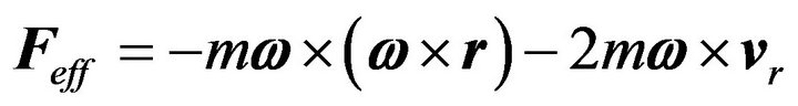
In a rotating coordinate system with angular velocity ω with respect to a fixed frame Newton’s 2nd law is [4],
 (1)
(1)
In this equation  is the effective acting force on a massive object of mass m. The subscripts f and r stand for fixed and relative frames, respectively.
  is composed of five potential distinct pieces: 1) F counts for the forces such as gravity, and friction, 2) the second term is the force due to the translation of the frame, 3) the third term arises from the nonuniform rotation of the rotating frame, 4) the fourth term is the centrifugal force and 5) the fifth term is the Coriolis force.
Applying Equation (1) to scenarios of interest simplifies its application, we consider a case where the rotating frame turns uniformly; this drops off the third term. The second term for a stationary observer is inoperative. One of the objectives of this study is to analyze the motion of an object for frictionless surfaces; this eliminates the first term. With these parameters Equation (1) sustains only the last two terms. Later on for the second phase of our analysis by turning on the friction we revive the first term. For time being for the scenario of interest Equation (1) reads
 (2)
(2)
For the rotating frame we consider a disk spinning about a fixed vertical axis. Utilizing for angular velocity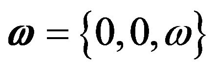 , the position vector
 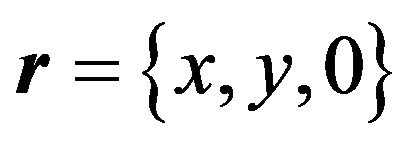 and its associated velocity
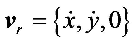 , Equation (2) yields,
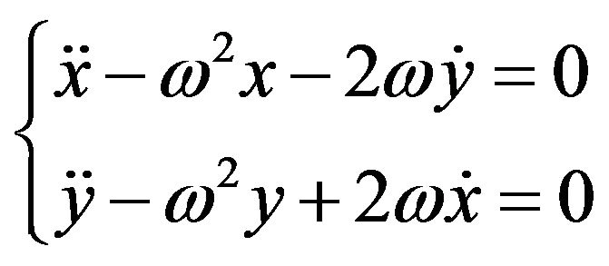 (3)
(3)
This is a set of coupled partial differential equations. We defer its solution to the next section. In pursue of our objective we now consider a scenario where a point-like charged particle is projected in a magnetic field. To put these two scenarios in the same footing, in a stationary coordinate system we set the magnetic field along a vertical axis;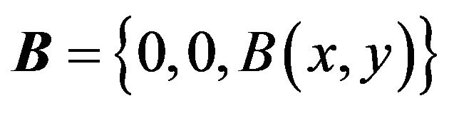 . A particle with a charge q projected in this field acquires a velocity
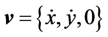 , and experiences a force
 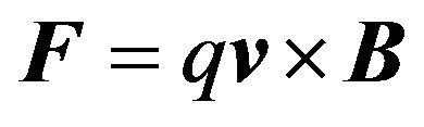 [3]. These parameters yield the equations of motion,
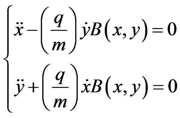 (4)
(4)
This also is a set of coupled partial differential equations. Here again we defer the solution to the next section. Aside from subtle detailed differences Equations (3) & (4) have a number of similarities. For instance Equation (3) for a small reduces to identical format of Equation (4). And most striking the angular velocity dependent coefficients in Equation (3) are similar the ones in Equation (4). In other words, because of these similarities one expects kinematic similarities as well. More on this in the next section.
3. Detailed Analysis
To qualify the observations of the previous section here we present their quantitative version. For instance it is instructive to solve, graphically display and compare the trajectories of these two scenarios under similar circumstances. First we note the set of Equation (3) for a chosen constant value can trivially be solved by combining the two independent variables {x, y} in one complex variable, z = x + iy. This reduces the two coupled equations in one,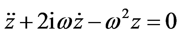 . The solution of this equation for a chosen set of initial conditions yields {x(t), y(t), 0}. Alternatively, one may apply CAS and solve Equation (3) numerically. On the other hand Equation (4) for a homogeneous magnetic field B has a trivial solution conducive to a circular trajectory. However, for most inhomogeneous fields is not analytically solvable; a numeric solution is required. Henceforth, for both scenarios we apply a numeric schematic solving the needed equations. The software of personal preference is Mathematica V9.0. In solving Equation (3) it appears the only explicit variable parameter is ω. However, other implicit parameters such as the initial speed and the orientation of the initial velocity play crucial roles as well. For the second scenario, as discussed in the previous section asides from variation of the initial velocity of the projected particle, the strength of the magnetic field is crucial as well. For 2D cases the inhomogeneity of the field is controlled with the functional format of the field, B(x,y). As such, in our analysis we have introduced three intuitively sound inhomogeneous fields. The interested reader may readily try out different inhomogeneities.
For the secondary objective we generalize the analysis by including a retarding force such as friction. Inclusion of this force turns on the first term of Equation (1). Substituting for ,
, 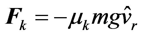 with
with  being the coefficient of kinetic friction Equation (3) modifies, yielding,
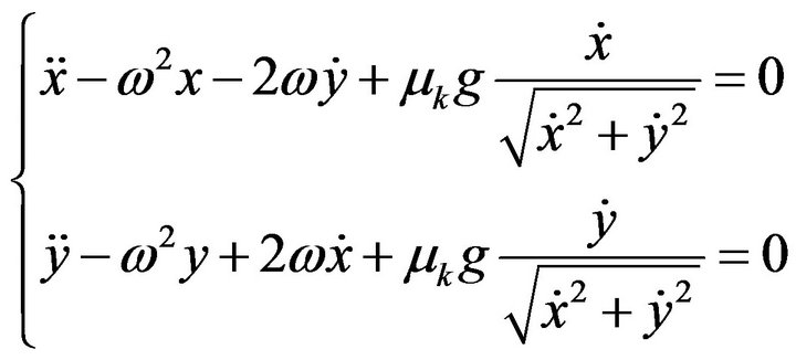 (5)
(5)
One look at Equation (5) qualifies the wisdom of having decided to solve the equations of motion numerically!
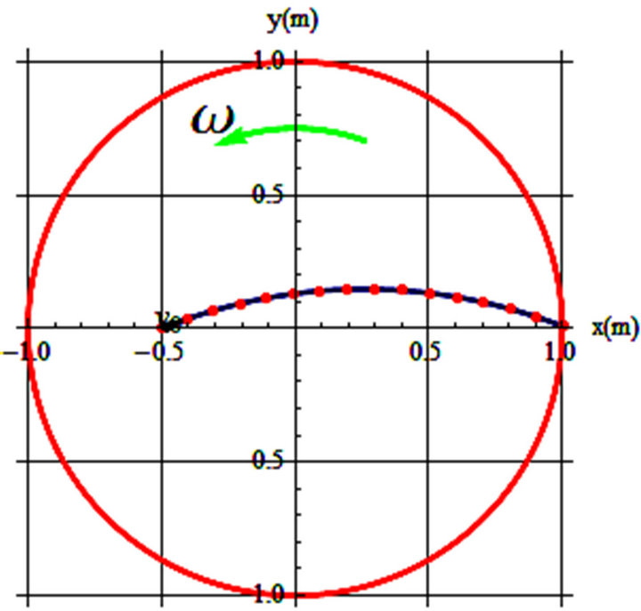
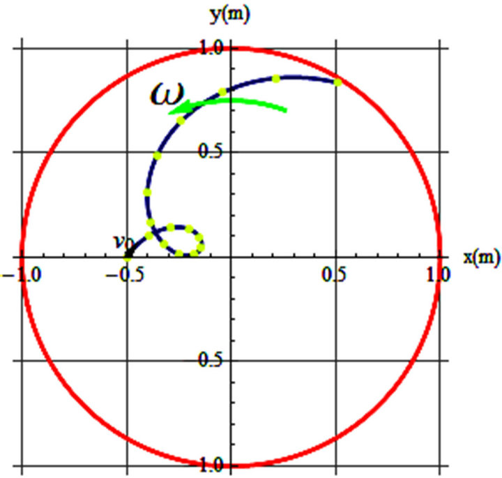
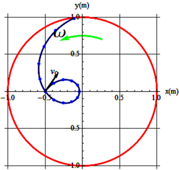
To display the trajectories observed on a rotating frame, first we consider the frictionless cases. Parameters conducive to the trajectories are captioned with the graphs. In these graphs the rotating frame is a disk of a one meter radius circle (shown in red) that turns counter clockwise with the shown ω-arrow. The initial position of the object is {x, y} = {–0.5, 0} and  is shown with its specifications printed at the bottom of each graph.
Figures 1-3 are display of the trajectories corresponding to the parameters printed in the captions. θ is the orientation of the initial velocity w/x-axis and t’s are the time the projectile stays on the spinning disk before separating from the disk.
The blue curves are the trajectories of the sliders on a frictionless horizontal turning table with its angular velocity aligned with the z-axis emerging from the paper. Our analysis reveals the general features of the trajectories are very sensitive to small changes of initial and angular velocity. As one may imagine there are countless possibilities for all various trajectories.
Now we focus our attention to the trajectories in a magnetic field. Solving Equation (4) is conducive to tra-
 (a)
(a)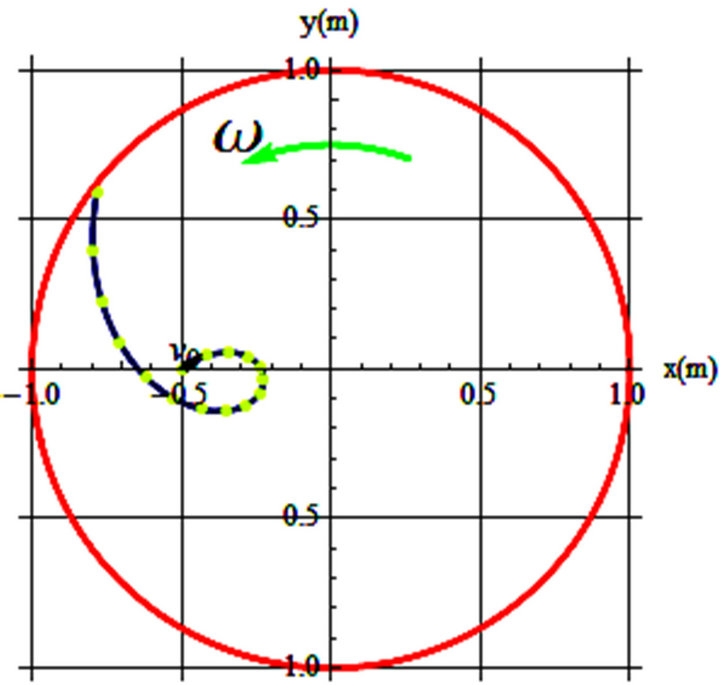 (b)
(b)
Figure 1. (a) v0 = 0.2 m/s, θ = 22˚, ω = 0.05 rad/s, t = 7.7 s; (b) v0 = 0.2 m/s, θ = 36˚, ω = 0.4 rad/s, t = 7.7 s.
 (a)
(a)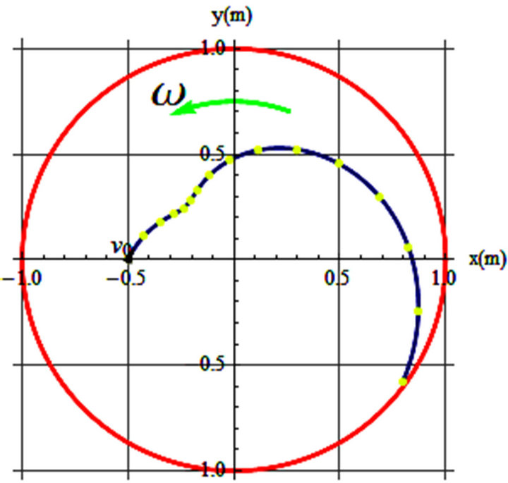 (b)
(b)
Figure 2. (a) v0 = 0.2 m/s, θ = 55˚, ω = 0.4 rad/s, t = 12 s; (b) v0 = 0.15 m/s, θ = 65˚, ω = 0.4 rad/s, t = 14.9 s.
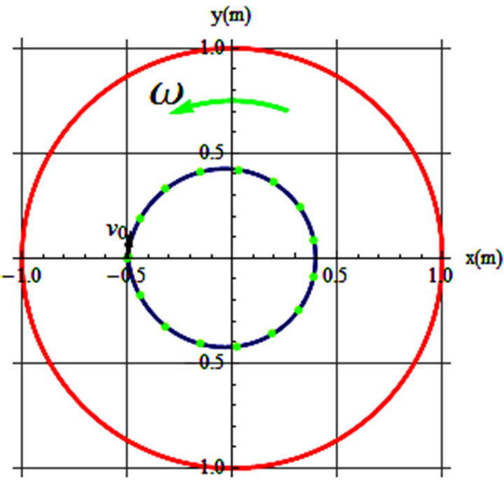
jectories. To begin with we consider a uniform field. As it is well known [2,3] a positively charged particle projected perpendicularly in the field circulates about the field; Figure 4 depicts one such trajectory. Orientation of the field emerging from the paper is symbolized by Circle-Dot. The field fills the 1 × 1 m square area; however, we confine the trajectories within the circular red circle. The trajectory is a circular blue clockwise loop; orientation of the initial velocity is shown as well.
By displaying this figure we are qualifying one of our objectives; that is, the trajectories depicted in Figures 3(a) and 4 are exactly the same. Without knowing the parameters that are conducive to these graphs one would not know whether they are the trajectories of a mechanical object in a rotating frame or of a magnetic field. In other words, the impact of the angular velocity in a rotating frame is equivalent to the impact of the magnetic field in a stationary one.
To distort the homogeneity of the magnetic field we
 (a)
(a)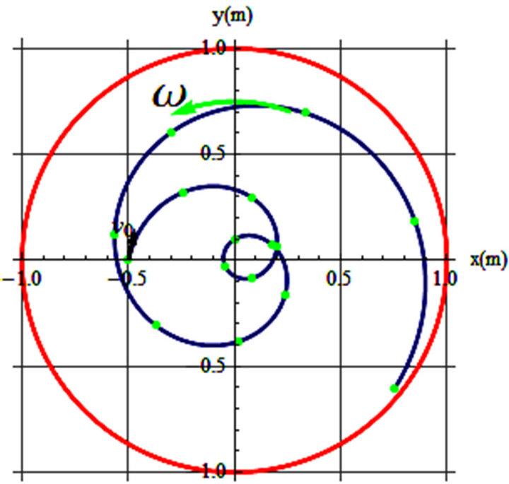 (b)
(b)
Figure 3. (a) v0 = 0.3 m/s, θ = 83˚, ω = 0.5 rad/s, t = 10 s; (b) v0 = 0.35 m/s, θ = 78˚, ω = 0.67 rad/s, t = 20 s.
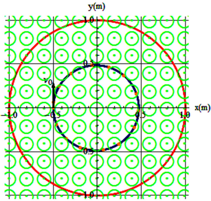
Figure 4. v0 = 0.68 m/s, θ = 90˚, B = 1.4 T, t = 53 s.
introduce three different classes of coordinate dependent fields 1) x-dependent, 2) y-dependent and 3) x-y dependent. The functional format of each field in real-life would depend on the needed application. Merely for theoretical interest we consider cases such as: xn, yn and (xy)n with n is a positive real number. Trajectories depicted in Figure 5 are due to x-dependent fields, e.g. B(x) = B0x1.5 and B(x) = B0x2. Parameters conducive to these trajectories are given in the captions.
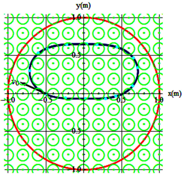
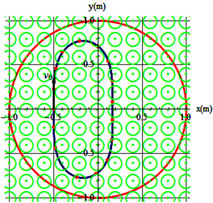
The localized stable elliptical trajectory in Figure 5(a) is due to B(x) = 4.8x1.5 Tesla. The trajectory depicted in Figure 5(b) is due to B(x) = 5.4x2 Tesla. Trajectories depicted in Figure 6 are y-dependent fields; the field is given by B(y) = B0y2. Parameters conducive to these trajectories are given in the captions.
Both trajectories are associated with the same field B(y) = 5.4y2 Tesla. The relevant differences are due to the initial velocities.
Lastly, for the 3rd class we consider symmetrical inhomogeneities on the x-y plane, e.g.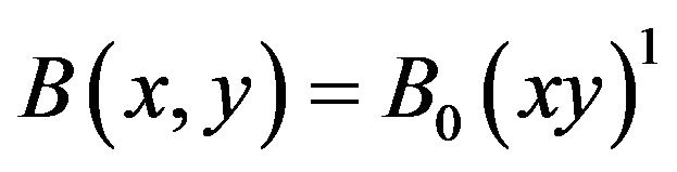 . Under the influence of one such field a projected charged
 (a)
(a)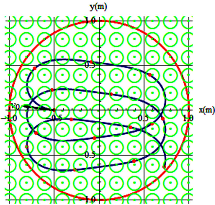 (b)
(b)
Figure 5. (a) v0 = 0.83 m/s, θ = 156˚, B = 4.8(x)1.5, t = 12 s; (b) v0 = 0.83 m/s, θ = 172˚, B = 5.4(x)2, t = 12 s.
 (a)
(a)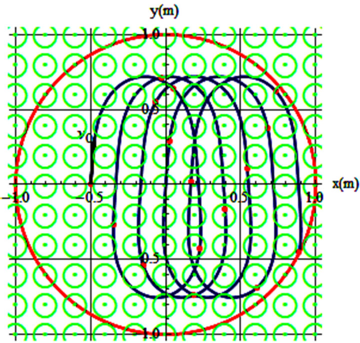 (b)
(b)
Figure 6. (a) v0 = 0.83 m/s, θ = 90˚, B = 5.4(y)2, t = 12; (b) v0 = 0.872 m/s, θ = 86˚, B = 5.4(y)2, t = 23 s.
particle with the initial velocity  results in the shown trajectory. As one may imagine there are countless trajectories corresponding to the chosen values of n, and the specifications of the initial velocities. Figure 7 is a display of one such case. This localized multiloop trajectory is a result of firing a positively charged particle with initial velocity
  in a 6.0 Tesla inhomogeneous field. The field retains the particle at least for about 23 s.
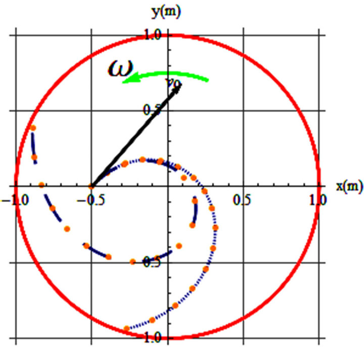
For the sake of curiosity we hunt for a set of parameters conducive to almost similar trajectories in the rotating frame and an inhomogeneous magnetic field. Figure 8 is one such case. Here again without knowing the parameters used for each plot one would have a challenging time identifying the causes: meaning, each of these trajectories could have been generated either in a rotating frame or in an inhomogeneous magnetic field. The latter cause along with Figure 8 is a quantified generalization of our main objective.

Figure 7. v0 = 0.57 m/s, θ = 90˚, B = 6(xy)1, t = 23 s.
 (a)
(a)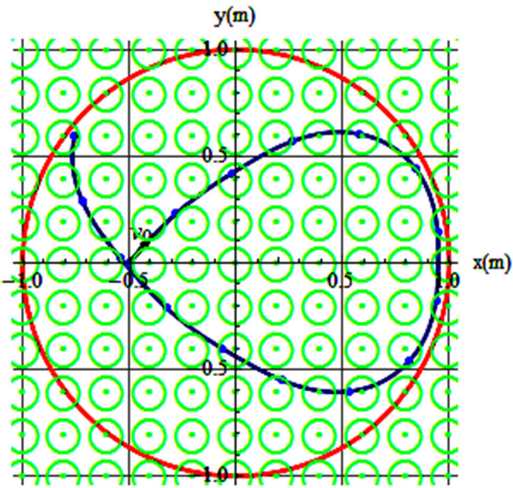 (b)
(b)
Figure 8. (a) v0 = 0.7 m/s, θ = 55˚, ω = 1.21 rad/s, t = 3.7 s; (b) v0 = 0.4 m/s, θ = 50˚, B = 1.8(xy)0.7, t = 12 s.
The secondary objective is to depict the impact of friction on the trajectories of rotating frames. As pointed out in the Detailed Analysis Section, by including friction the equations of motion are modified; these are given by Equation (5). The numeric solution of these equations for chosen initial conditions is conducive to the trajectories of interest. Plots shown in Figure 9 are comparative displays of trajectories with and without friction. The parameters of each paired curves are given in the captions.
The short-dashed curve in Figure 9(a) corresponds to frictionless trajectory and the long-dashed curve corresponds to the trajectory with friction. In drawing these trajectories the combined parameter namely  is essential rather than the
  by itself. For instance a typical coefficient of kinetic friction
  with a
  gives
gives . As such, for the same initial velocity and angular velocity the rough surface
 (a)
(a)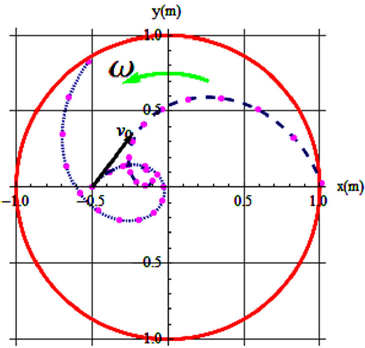 (b)
(b)
Figure 9. (a) Parameters of the left graph are: v0 = 2 m/s, θ = 49˚, ω = 2.2 rad/s, mkg = 0.0, t = 1.05 s, mkg = 1.0, t = 2.25 s; (b) Parameters of the right graph are: v0=1. m/s, θ = 53°, ω = 1.66 rad/s, mkg = 0.3, t =2.5, and t = 4.4 s.
bends the trajectory more pronouncedly, keeping the object on the frame longer, i.e. the short-dashed curve with t =1.05 s vs. long-dashed curve with t = 2.25 s. Similarly, the short-dashed curve in Figure 9(b) corresponds to the frictionless surface, while the long-dashed curve is associated with . Here the surface is smoother but the initial speed and the angular velocity are slower resulting a shorter life-time, i.e. t = 4.45 s vs. t = 2.25 s, respectively.
4. Conclusion and Remarks
We have two targeted objectives. First we wish to demonstrate that impact of the angular velocity in a rotating frame is the same as the impact of the magnetic field in a stationary frame. We achieve this goal qualitatively as well as quantitatively. The secondary objective is to extend quantitatively the analysis of the first objective including the impact of retarding forces such as friction. To quantify the impact of friction, we rely on the application of a CAS, specifically Mathematica. We solve the coupled non-linear partial differential equations and display comparatively the cases without vs. with friction cases, receptively. Not reported are the extensive Mathematica codes automating the integration of solutions of the equations and their graphic output. Also because of the space limitation only a handful of graphs are included in this article. The interested reader may apply the guided outlines extending the computations.
REFERENCES
- Mathematica, “A General Computer Software System and Language Intended for Mathematical and Other Applications,” V9.0, Wolfram Research, Champaign, 2013.
- https://www.boundless.com/physics/magnetism/motion-charged-particle-in-magnetic-field-2/circular-motion-5 https://ilt.seas.harvard.edu/images/material/493/235/Ch28n32v2.24.pdf
- J. D. Jackson, “Classical Electrodynamics,” 3rd Edition, Wiley, New York, 1998.
- S. T. Tronton and J. B. Marion, “Classical Dynamics of Particles and Systems,” 5th Edition, Cengage Learning, Independence, 2008.
- A. P. French, “Newtonian Mechanics,” W. W. Norton, New York, 1971, pp. 528-529.
- G.-G. Coriolis, “Sur les Équations du Mouvement Relatif des Systèmes de Corps,” Journal de l’Ecole Royale Polytechnique, Vol. 15, 1835, pp. 144-154.
- R. P. Feynman, R. B. Leighton and M. Sands, “The Feynman Lectures on Physics, Vol. 1,” Addison-Wesley, Redwood City, 1989, pp. 19-8-19-9.