Journal of Electromagnetic Analysis and Applications
Vol.4 No.1(2012), Article ID:17150,12 pages DOI:10.4236/jemaa.2012.41005
Modeling of Antenna for Deep Target Hydrocarbon Exploration
![]()
1Fundamental and Applied Sciences Department, Universiti Teknologi PETRONAS, Tronoh, Malaysia; 2Electrical Electronics Engineering Department, Universiti Teknologi PETRONAS, Tronoh, Malaysia.
Email: *noorhana_yahya@petronas.com.my
Received November 15th, 2011; revised December 16th, 2011; accepted December 28th, 2011
Keywords: Electromagnetic; Hydrocarbon; SBL; Antenna; CST
ABSTRACT
Nowadays control source electromagnetic method is used for offshore hydrocarbon exploration. Hydrocarbon detection in sea bed logging (SBL) is a very challenging task for deep target hydrocarbon reservoir. Response of electromagnetic (EM) field from marine environment is very low and it is very difficult to predict deep target reservoir below 2 km from the sea floor. This work premise deals with modeling of new antenna for deep water deep target hydrocarbon exploration. Conventional and new EM antennas at 0.125 Hz frequency are used in modeling for the detection of deep target hydrocarbon reservoir. The proposed area of the seabed model (40 km ´ 40 km) was simulated by using CST (computer simulation technology) EM studio based on Finite Integration Method (FIM). Electromagnetic field components were compared at 500 m target depth and it was concluded that Ex and Hz components shows better resistivity contrast. Comparison of conventional and new antenna for different target depths was done in our proposed model. From the results, it was observed that conventional antenna at 0.125 Hz shows 70%, 86% resistivity contrast at target depth of 1000 m where as new antenna showed 329%, 355% resistivity contrast at the same target depth for Ex and Hz field respectively. It was also investigated that at frequency of 0.125 Hz, new antenna gave 46% better delineation of hydrocarbon at 4000 m target depth. This is due to focusing of electromagnetic waves by using new antenna. New antenna design gave 125% more extra depth than straight antenna for deep target hydrocarbon detection. Numerical modeling for straight and new antenna was also done to know general equation for electromagnetic field behavior with target depth. From this numerical model it was speculated that this new antenna can detect up to 4.5 km target depth. This new EM antenna may open new frontiers for oil and gas industry for the detection of deep target hydrocarbon reservoir (HC).
1. Introduction
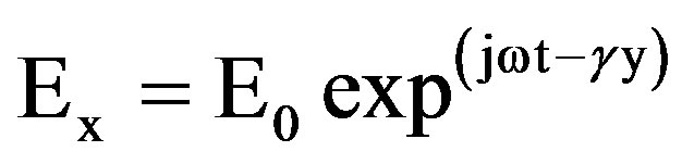
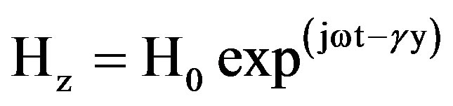
Sea bed logging is an application of control source electromagnetic method which is used to locate an oil reservoir beneath the sea floor by measuring electromagnetic fields [1-4]. In typical control source method a horizontal electric dipole antenna is towed by a surface vessel at a short distance 30 m above from the sea floor [5-7]. Dipole antenna transmits very low frequency electromagnetic waves with frequency ranges from 0.25 Hz - 10 Hz due to low frequency transmitted energy propagates down through the subsurface [8-10]. Low frequency electromagnetic waves attenuate more in the conductive layer and less in the resistance layer due to the skin depth. In a large resistive layer such as hydrocarbon electromagnetic energy flows along the reservoir (described as guided wave) is detected by the stationary sea floor electric or magnetic field detectors which are deployed on the sea floor. Control source electromagnetic method depends on the resistivity of the hydrocarbon and surrounding sediments. Hydrocarbon in the sea bed has resistivity of few tens to hundred ohm meter (30 Ωm - 500 Ωm), sea water (0.5 Ωm - 2 Ωm) while all other layers including sediments in the sea have resistivity (1 Ωm - 2 Ωm) [11-17]. In deep water the air wave effect is negligible so the wave guided back from the hydrocarbon can predict the presence of hydrocarbon [18]. Target depth is also very important in sea bed logging. Frequency and offset plays an important role to determine target depth. Shallow targets shows measurable response at near offset with high frequency where as deep targets at large offset with low frequency. G. Michael Hoversten reports that simulated oil-water contact at 2 km depth below the sea floor shows a response below the expected noise levels. The resistivity model in which maximum target depth response measured was 3 km for 8 km offset [19]. Multiple frequency range of electromagnetic waves is used to improve control source electromagnetic data for deep target hydrocarbon reservoir. Deep target having variable size and depth can cause the risk factor so high and low frequency reduces this risk factor. Deep water field survey in Nigeria two fundamental frequencies (0.05 Hz and 0.25 Hz) with higher frequency are used which shows very promising survey results. For shallow target depth 0.25 Hz frequency and the first two harmonics is useful to detect the thin resistive hydrocarbon reservoir. Low frequency (0.05 Hz) data provide useful information about 2 km resistivity background model. This wide range of multiple frequencies is used to reduce the drilling risk factor [20]. Direct detection of hydrocarbon which is deeply buried can be done by subsea EM sounding technique. Survey was done across TWGP, Norway offshore and they found the target at the depth of 1100 m below the sea floor was reported [21]. Transmitter height changing above the sea floor was investigated in a noise model and also included the data which create uncertainty by changing the transmitter height. Inversion of the data with multilayers and four layers models was done. It was observed that this model can detect the resistive layer at a depth of 1500 - 1600 m below the sea floor for control source CSEM electromagnetic method where as 2 km depth for seismic method [22]. Propagation of electromagnetic (EM) waves travelling in seawater can be predicted by using Maxwell’s equations. If the propagating of electromagnetic wave in the y direction then it can be described in terms of the electric field strength Ex and the magnetic field strength Hz [23].
 (1)
(1)
 (2)
(2)
 (3)
(3)
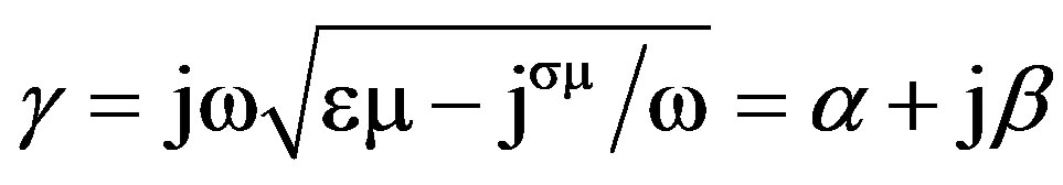
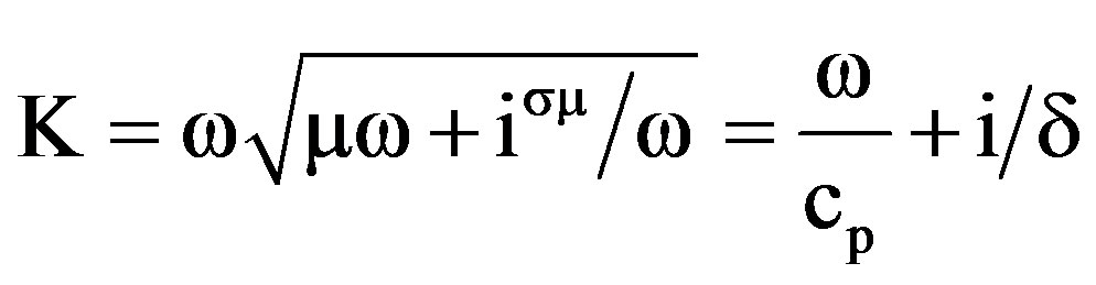
where (γ) is the propagation constant, (ε) permittivity, (μ) permeability, (σ) conductivity, α attenuation factor, β phase factor and ω = 2πf the angular frequency as given in Equation (3). Electromagnetic wave propagation can be described by a wave number K as given in Equation (4).
 (4)
(4)
where K is the wave number and  is the complex number, cp phase velocity and d is the skin depth. First term in Equation (4) inside the square root represent the displacement current and second term represent conduction current in Maxwell’s equation.
Numerical model is a very important to know the location hydrocarbon in sea bed logging. It can provide the information about the target depth at which target depth the electromagnetic wave signal provide information about hydrocarbon reservoir [24].
This work premise deals with the study of electromagnetic field components, conventional and new antenna electromagnetic field comparison for deep target hydrocarbon reservoir detection. New antenna electric field data of different curvatures is used for numerical model to know the exact target depth with this new antenna design.
2. Modeling Methodology
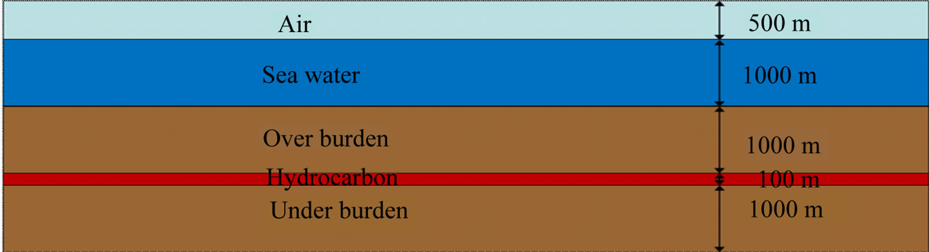
We use CST (Computer simulation technology) software for finite integration method (FIM). Computer simulation technology (CST) is used to discritize each Maxwell’s equations at low frequency to investigate the resistivity contrast. For finite integration technique, Computer simulation technology software is used as a tool for low frequency to solve any problem. FIM was used to detect deep target hydrocarbon below 3000 m from seafloor by using CST software. CST software was used to detect deep target hydrocarbon between 1000 m to 400 m underneath seabed. Model area was assigned as 40 ´ 40 km to replicate the real seabed environment with various target positions. Environment with and without hydrocarbon were also prepared for comparison purpose later. There were few steps involved in generating the CST simulated model. First step was to set parameters for aluminium antenna. In this case we used length of 270 m, frequency of 0.125 Hz and current of 1250 A. Second step was to set parameters for the model. Air thickness was set as 500 m, sea water depth of 2000 m, overburden thickness of 1000 m, hydrocarbon thickness of 100 m and under burden with their different conductivities and permeability values (Table 1). Thickness of the overburden was increased as the target depth varied gradually (every 250 m) from 500 m to 5000 m. Third step was to apply electric boundary conditions (Table 2). Fourth step was to run low frequency full wave solver to simulate sea bed model. The final step was post processing to generate the simulated data for results analysis at different target depths. Maxwell’s equations for magnetic and electric fields are used as a code in the software to get electric and magnetic field response with and without HC. Schematic diagram of proposed seabed model with CST simulated model is shown in Figure 1.
3. Results and Discussion
3.1. Electromagnetic Field Components Study
Electromagnetic field components response from hydrocarbon reservoir in sea bed logging is very important to show better resistivity contrast. In sea bed logging both electric and magnetic field sensors are placed on the sea floor to record the electromagnetic field data. Electromagnetic field data consists of three components i.e. (x, y,
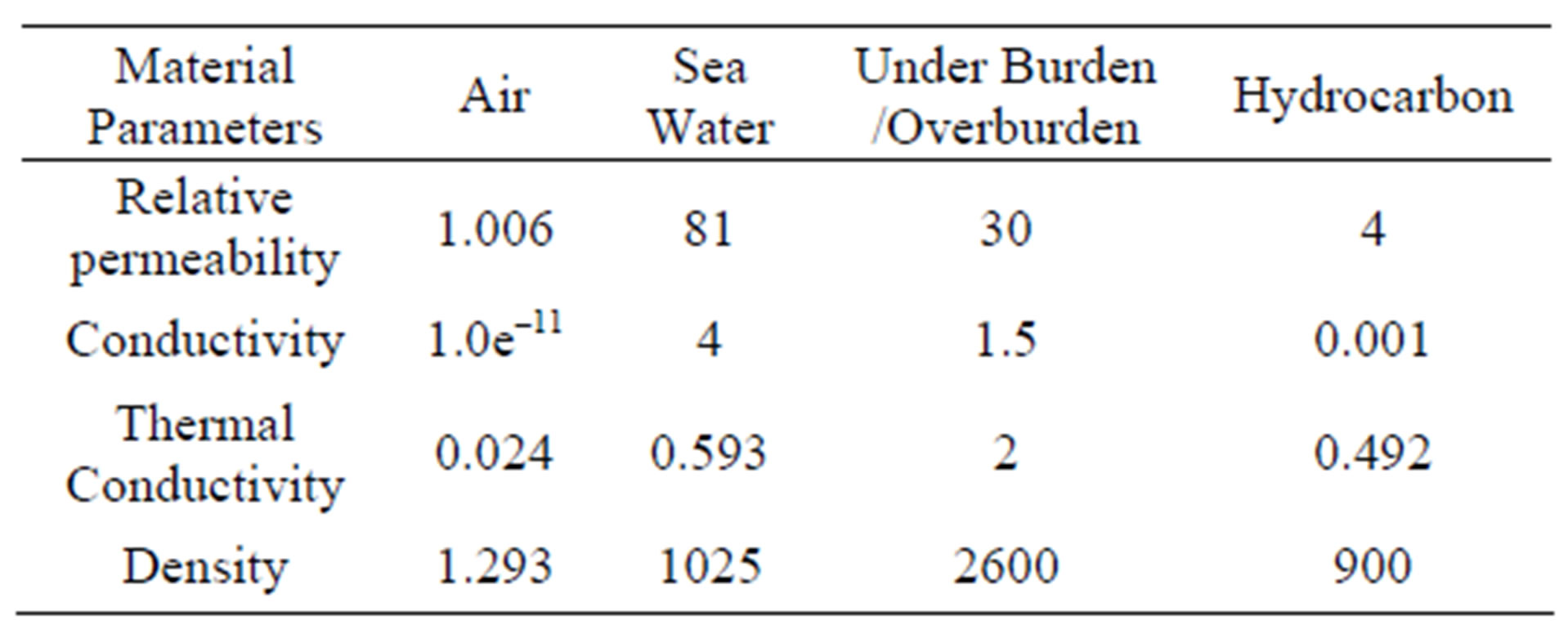
Table 1. Relative permittivity, conductivity values of air, sea water overburden/under burden and hydrocarbon.
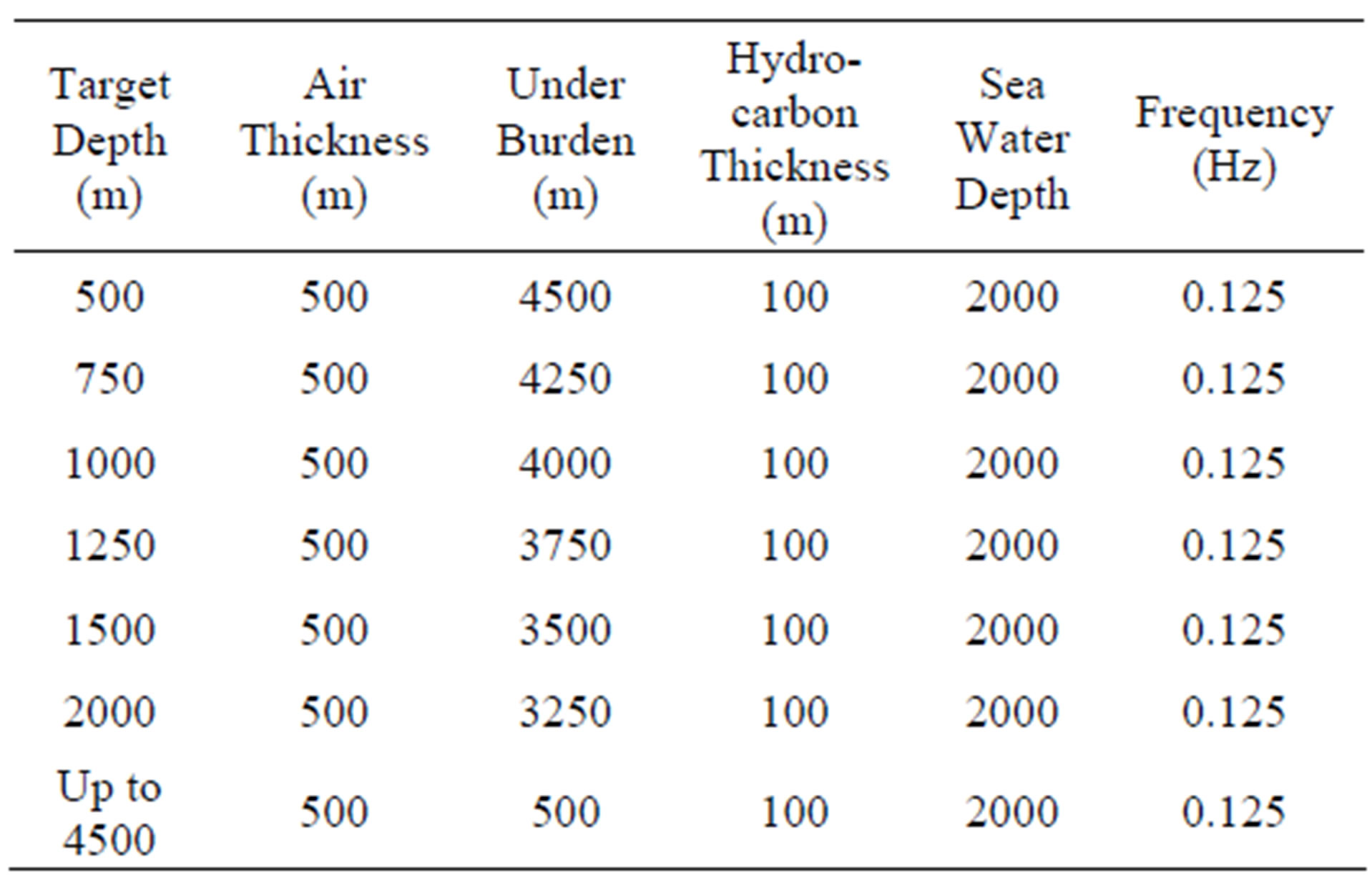
Table 2. Simulated model parameters with different resistive layers (air, sea water, overburden and under burden).
 (a)
(a) (b)
(b)
Figure 1. (a) Schematic diagram of proposed model and (b) CST simulated model.
and z). Choice of the electromagnetic field components depends on the electromagnetic waves propagation. All three components of electric field response were measured with conventional HED antenna within the proposed area (40 km ´ 40 km). Components study was done in deep water (2000 m) where no air waves effect take place. Comparison of E-field components is given in Figure 2. Ex component shows better E field response at 500 m target depth as compared to Ey and Ez.
Magnetic field components comparison was also done to know which component gave high magnetic field response with the presence of hydrocarbon reservoir. Magnetic field strength is although lower than the elec-
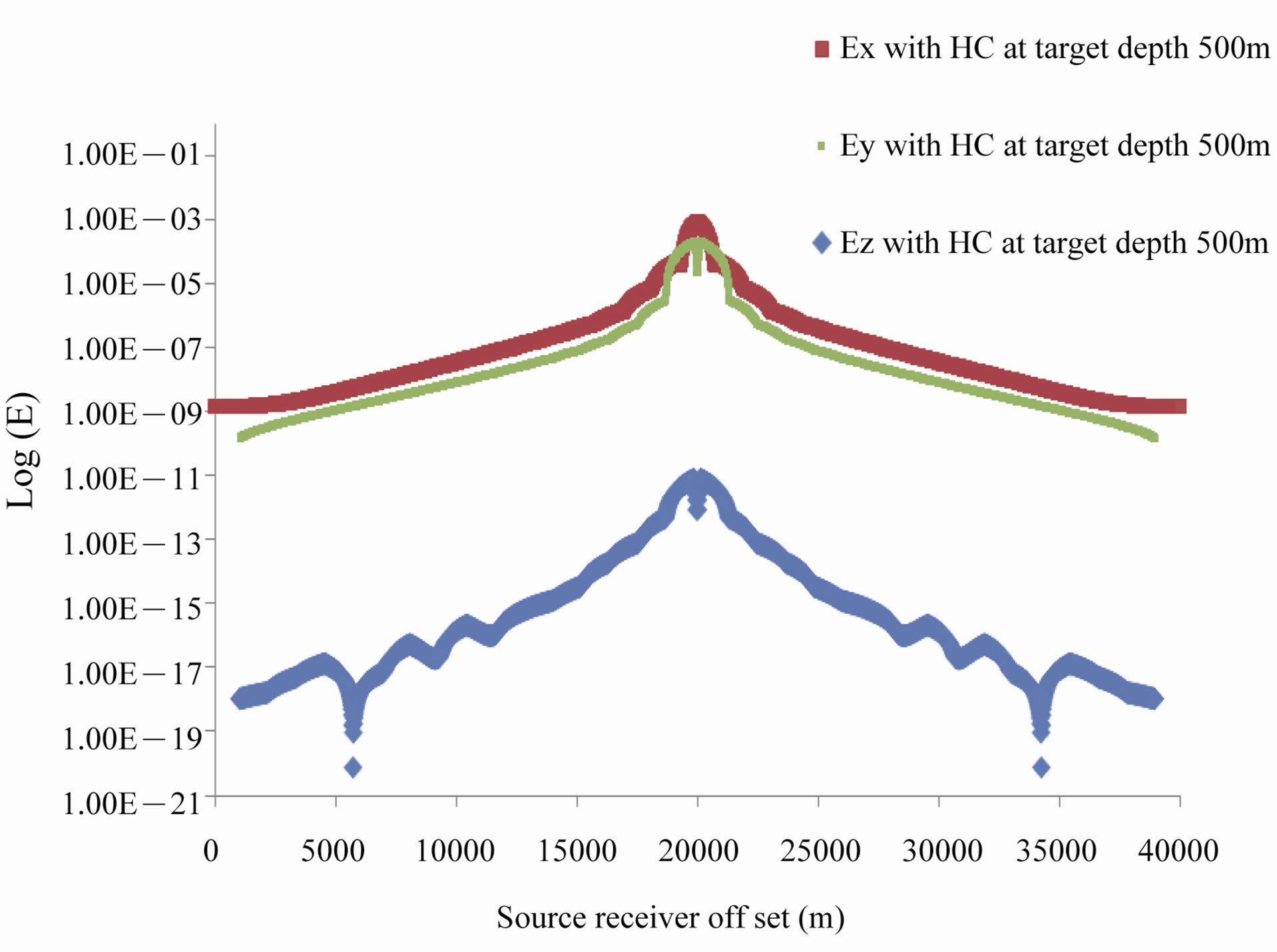
Figure 2. Comparison of E-filed components (Ex, Ey, Ez) response at 500 m target depth.
tric field strength but it is also very important for hydrocarbon prediction but only for shallow target where as for deep target the signal strength is very low which cannot be able to predict the presence of hydrocarbon reservoir. Magnetic field comparison is given in Figure 3. Bz component gave higher magnetic field response with the presence of hydrocarbon reservoir at 500 m depth.
H-field response was also analyzed at 500 m target depth is given in Figure 4. H-field response of all three components was recorded and plotted to know which component gave higher response. Hz component shows better response with the presence of hydrocarbon reservoir than Hx and Hy. Selection of E, B and H field components was done and it was conclude that Ex, Bz and Hz gave better delineation of hydrocarbon reservoir at 500 m target depth. Finally Ex, Bz and Hz electromagnetic field components were plotted as given Figure 5. Hz and Ex gave better delineation than Bz component. These two components were chosen for deep target hydrocarbon detection with straight and new antenna.
3.2. Straight Antenna MVO Results
Straight antenna magnitude verses offset data was plotted to compare with new antenna in full scale sea bed logging environment. Conventional antenna and new antenna length, frequency and model were kept same to check the performance of new antenna for deep water-deep target.
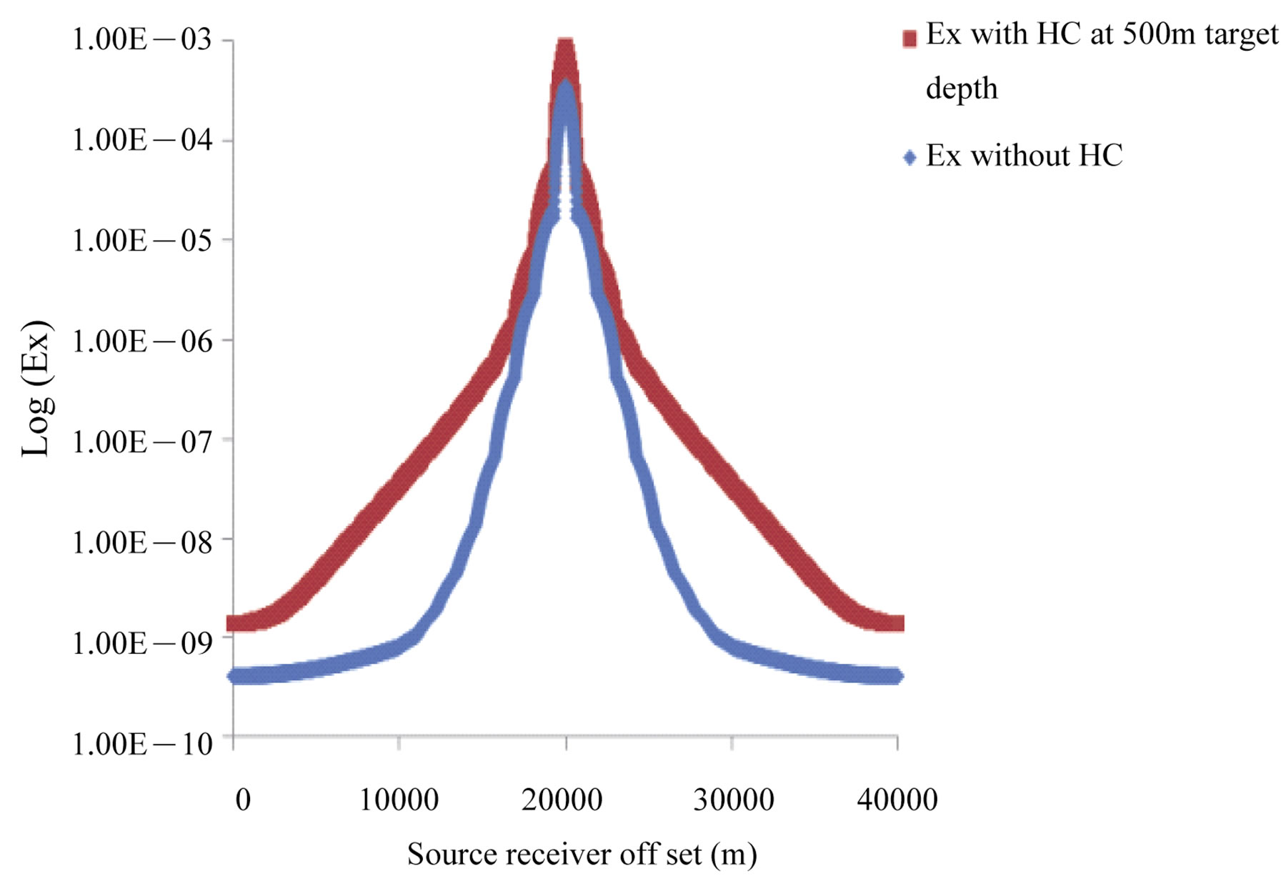
Straight antenna magnitude verses offset data was plotted by changing the target depth from 500 m until 2000 m. Ex field response with and without hydrocarbon was measured to know the exact target depth which can be detected by the straight HED antenna in deep water. At 500 m target depth straight antenna shows 70% resistivity contrast is given Figure 6(a). Target depth was varied from 500 m to 750 m but the simulated model total
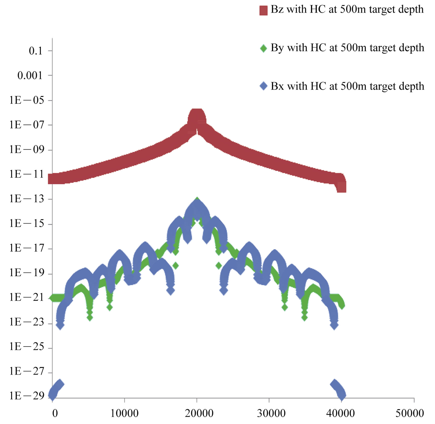
Figure 3. Comparison of B-filed components (Bx, By, Bz) response at 500 m target depth.
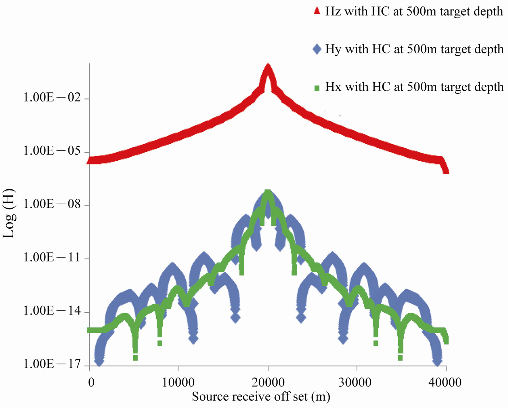
Figure 4. Comparison of H-field components (Hx, Hy, Hz) response at 500 m target depth.

Figure 5. Comparison of Hz, Ex and Bz field response at 500 m target depth.
 (a)
(a)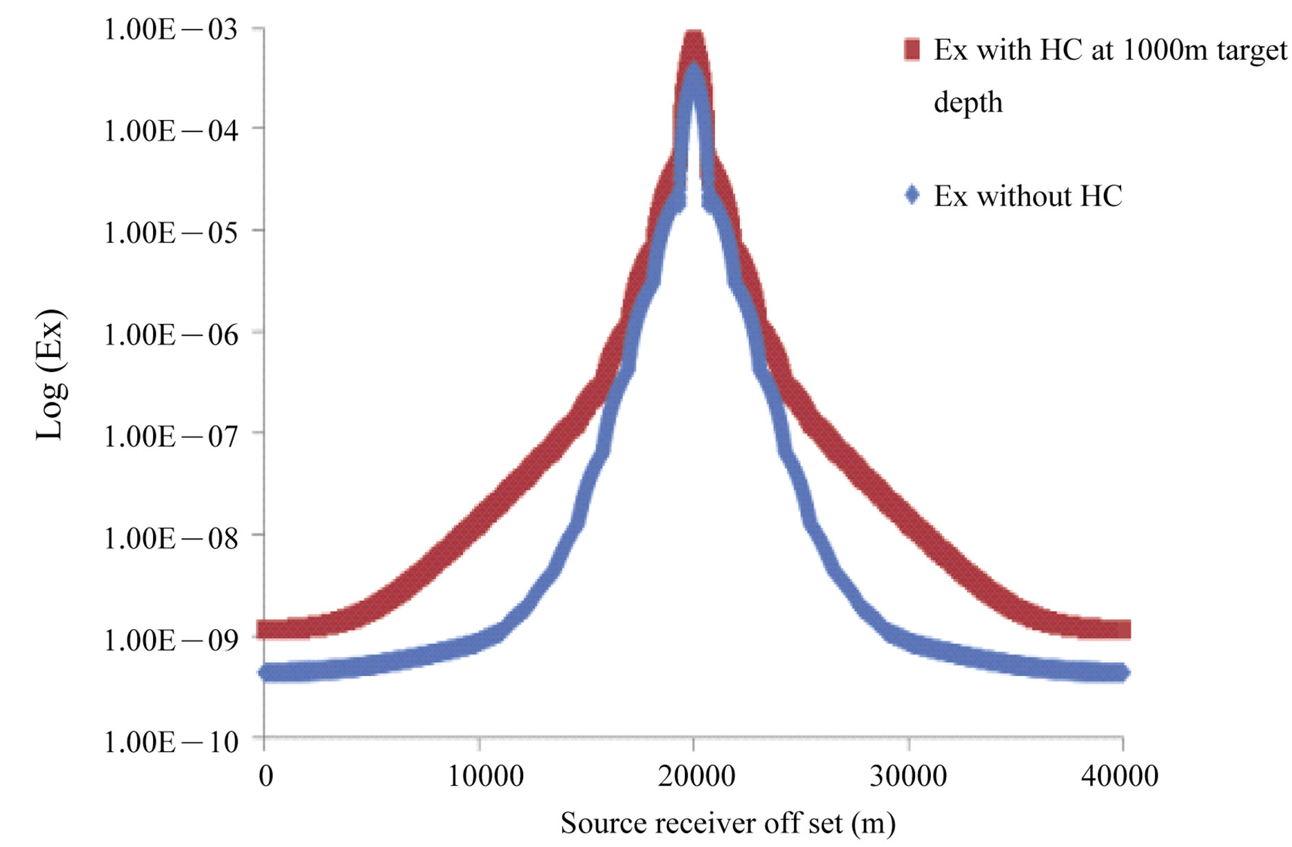 (b)
(b)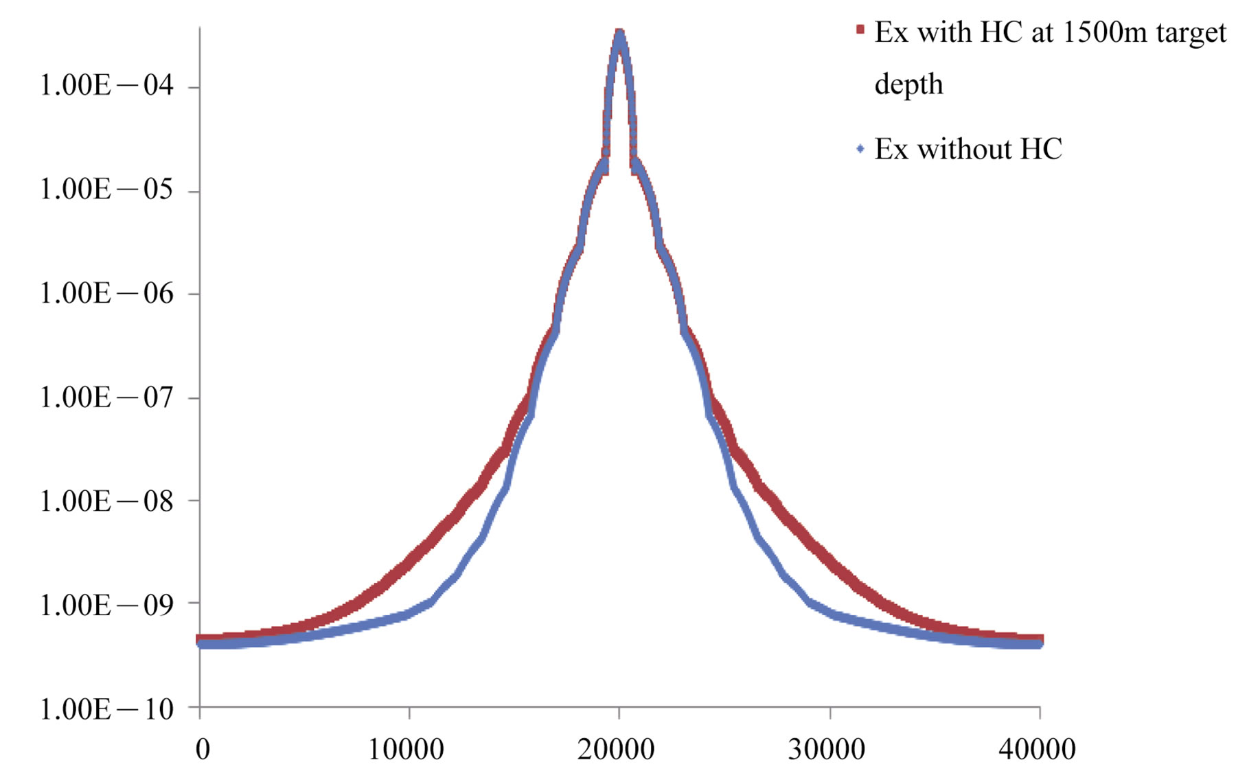 (c)
(c) (d)
(d)
Figure 6. Straight antenna Ex-field MVO with different target positions (a) 500 m; (b) 1000 m; (c) 1500 m; (d) 2000 m.
layers depth keep constant by reducing the under burden depth. Ex field response decreases by increasing the target depth due to the skin depth. At 750 m target depth resistivity contrast drops to 57% is shown Figure 6(b). Ex field response was measured until no hydrocarbon detected. It was analyzed that 42%, 26% and 12% difference with and without hydrocarbon at 1000 m, 1250 m and 1500 m respectively. Further target depth was decreased from 1500 m to 2000 m the difference between with and without hydrocarbon reservoir is 5% and 2% which is less than 10%. Straight antenna can detect up to 1500 m target depth below the sea floor because drilling risk factor is involved below 10%.
Hz field response was also measured with straight antenna to get better delineation of hydrocarbon reservoir. Analysis between Ex and Hz at 500 m target depth shows 16% better delineation of hydrocarbon reservoir than Ex field response. At 1500 m target depth Hz field response
was 12% higher than Ex field response. It was also conclude that Hz field shows 10% difference at 1750 m target depth. Magnetic field Hz component able to detect the hydrocarbon reservoir at 1750 m target depth where as Ex field response for 1500 m target depth respectively. Due to high H-field strength it can detect 250 m extra depth than Ex field response is given Figure 7. Below 2000 m strong electromagnetic signal strength is required for deep target hydrocarbon detection.
3.3. New Antenna MVO Results
Deep target detection is a challenging task in sea bed logging. Response from deep target hydrocarbon reservoir is very weak from straight antenna. The guided wave from the high resistive deep target has very low signal strength which is very difficult to predict the presence of hydrocarbon reservoir. A strong EM field is required and
 (a)
(a)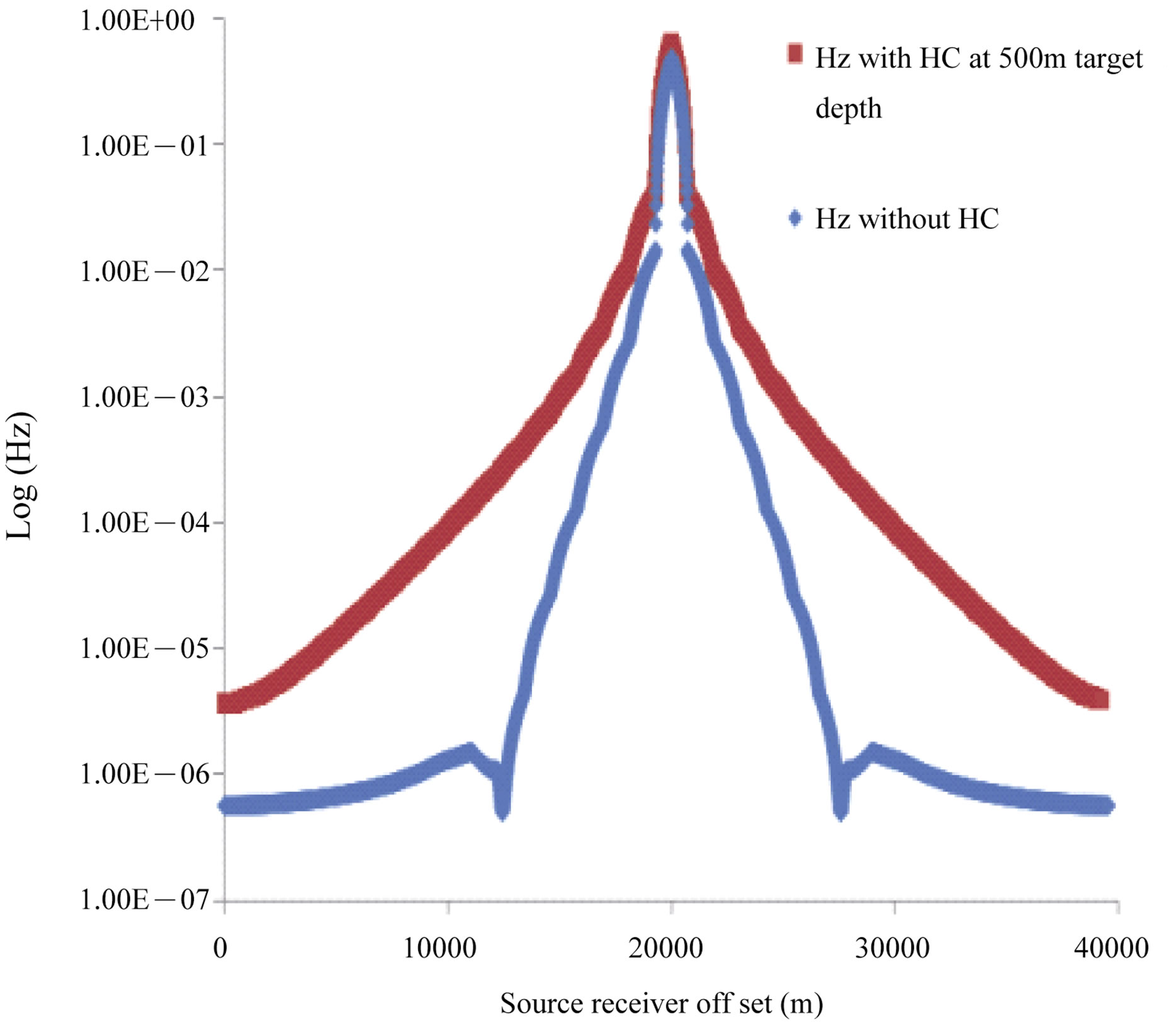 (b)
(b)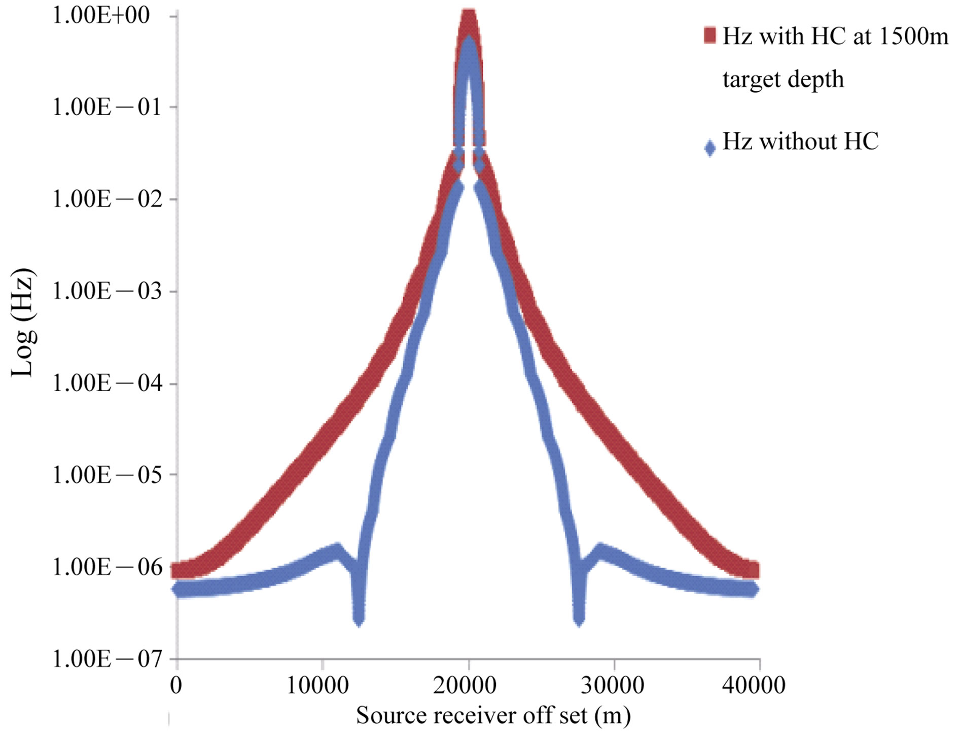 (c)
(c) (d)
(d)
Figure 7. Straight antenna Hz field MVO with different target positions (a) 500 m; (b) 1000 m; (c) 1500 m; (d) 2000 m.
some modification of the HED antenna is highly needed by the oil and gas industry to ensure deep target. To enhance the signal strength and focus more electromagnetic (EM) waves for deep target new antenna was simulated with and without the presence of hydrocarbon reservoir to check the performance of new antenna. The proposed area of the seabed model which was simulated by using CST (computer simulation technology) EM studio based on Finite Integration Method (FIM). New antenna has the ability to focus electromagnetic waves.
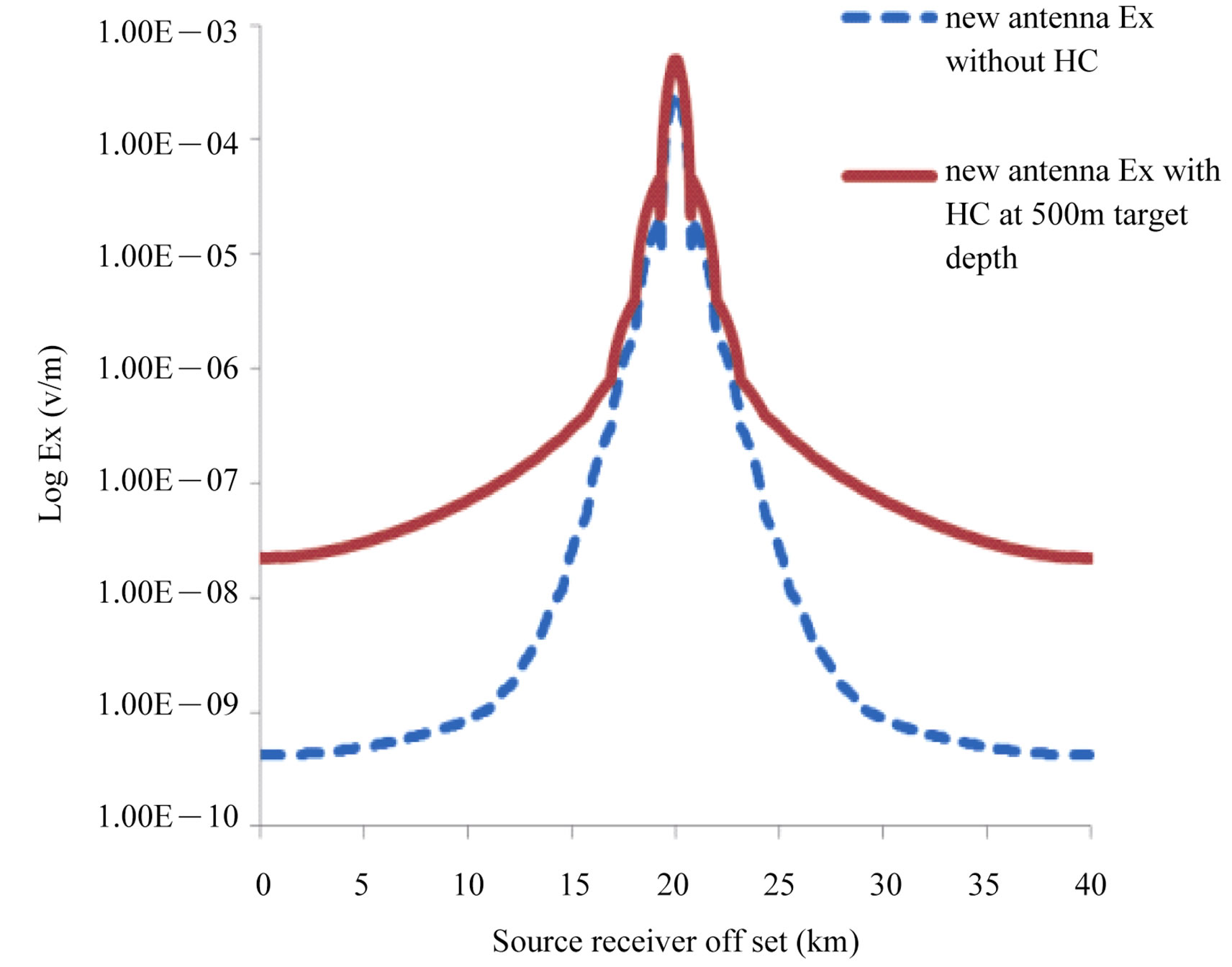
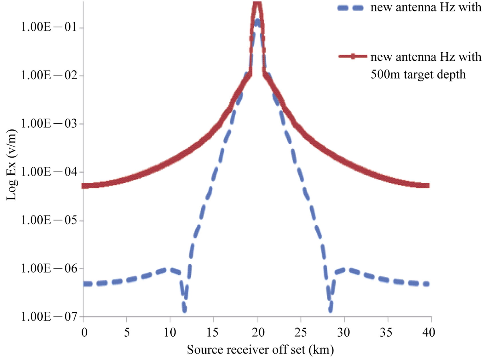
New antenna was used to get the magnitude verses offset (MVO) response for 4000 m target depth as given Figure 8. Solid lines indicate the response with presence of hydrocarbon where as dotted line represents without hydrocarbon response. It was analyzed that this new antenna shows 510% difference between the hydrocarbon or without hydrocarbon at 500 m target depth than straight antenna. This difference motivates to go for further target depth to predict the presence of high resistive layers hydrocarbon (HC). New antenna Ex field response shows 46% difference between with and without hydrocarbon resrvior at 4000 m target depth is given Figure 8. This
 (a)
(a)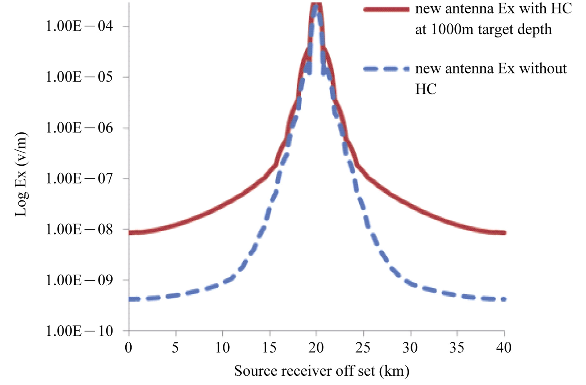 (b)
(b)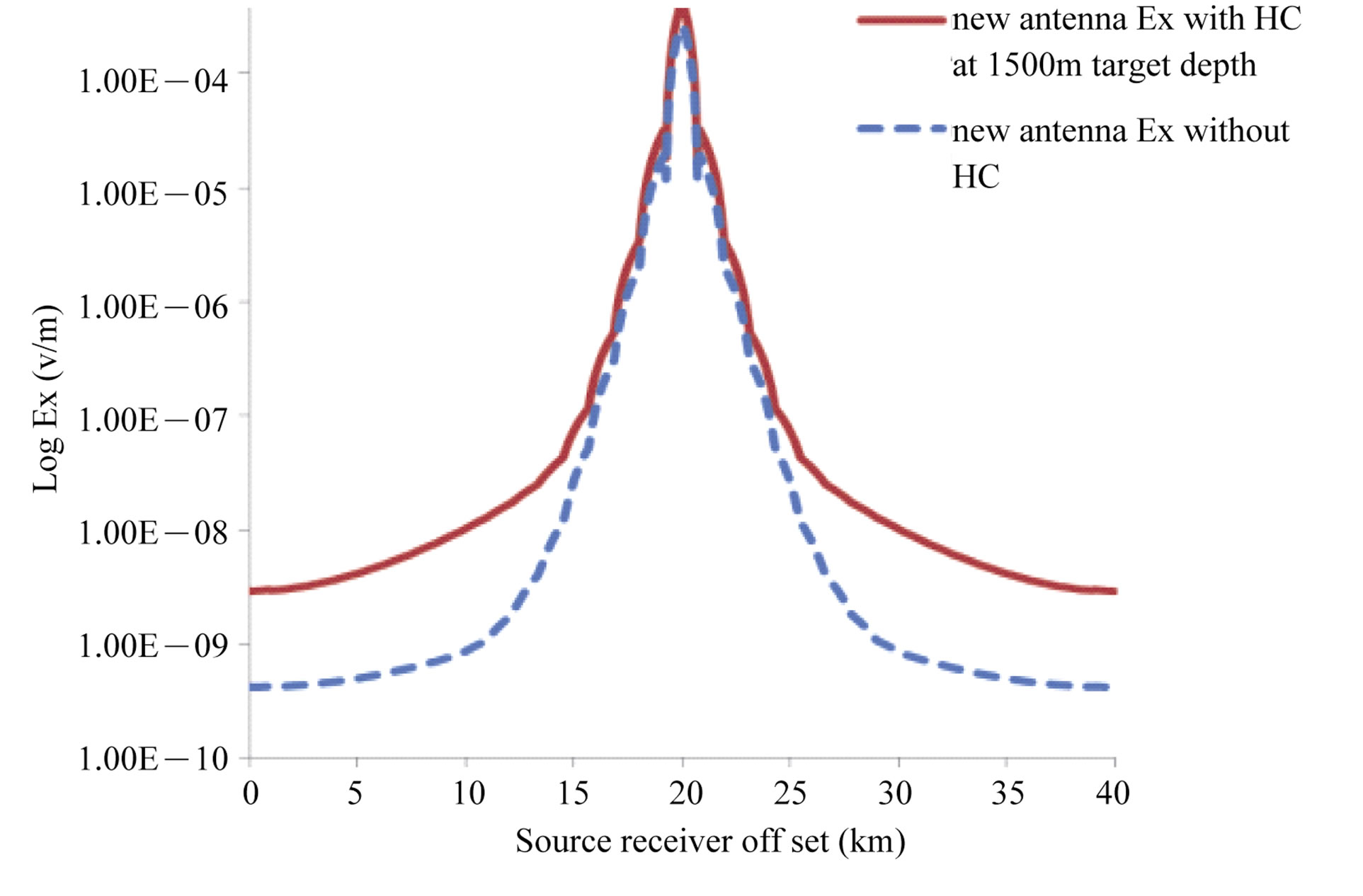 (c)
(c)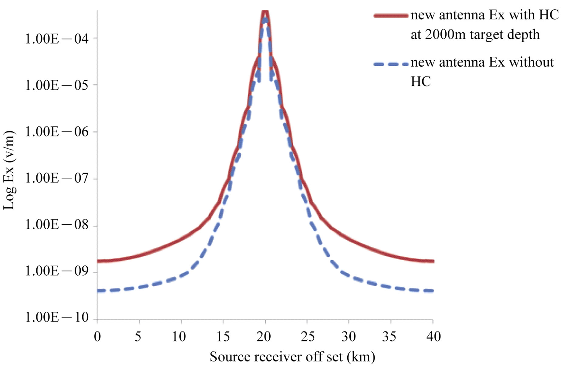 (d)
(d) (e)
(e)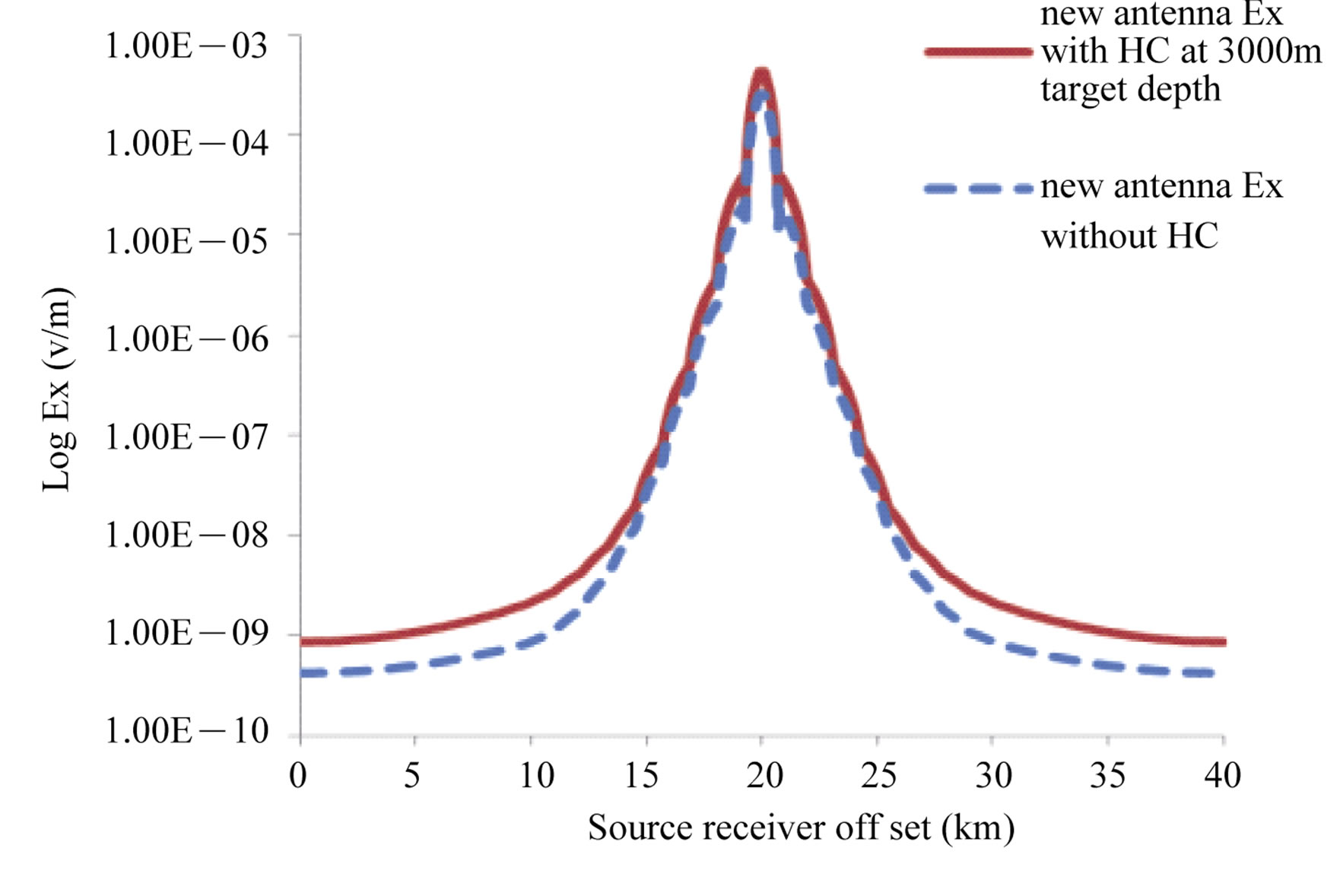 (f)
(f)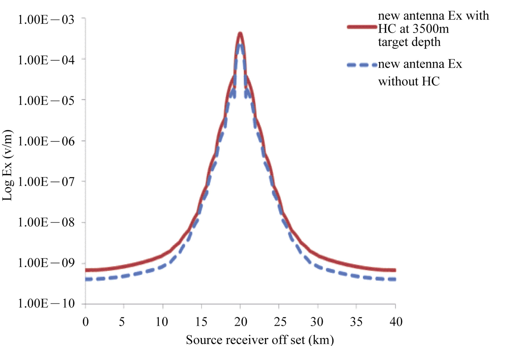 (g)
(g)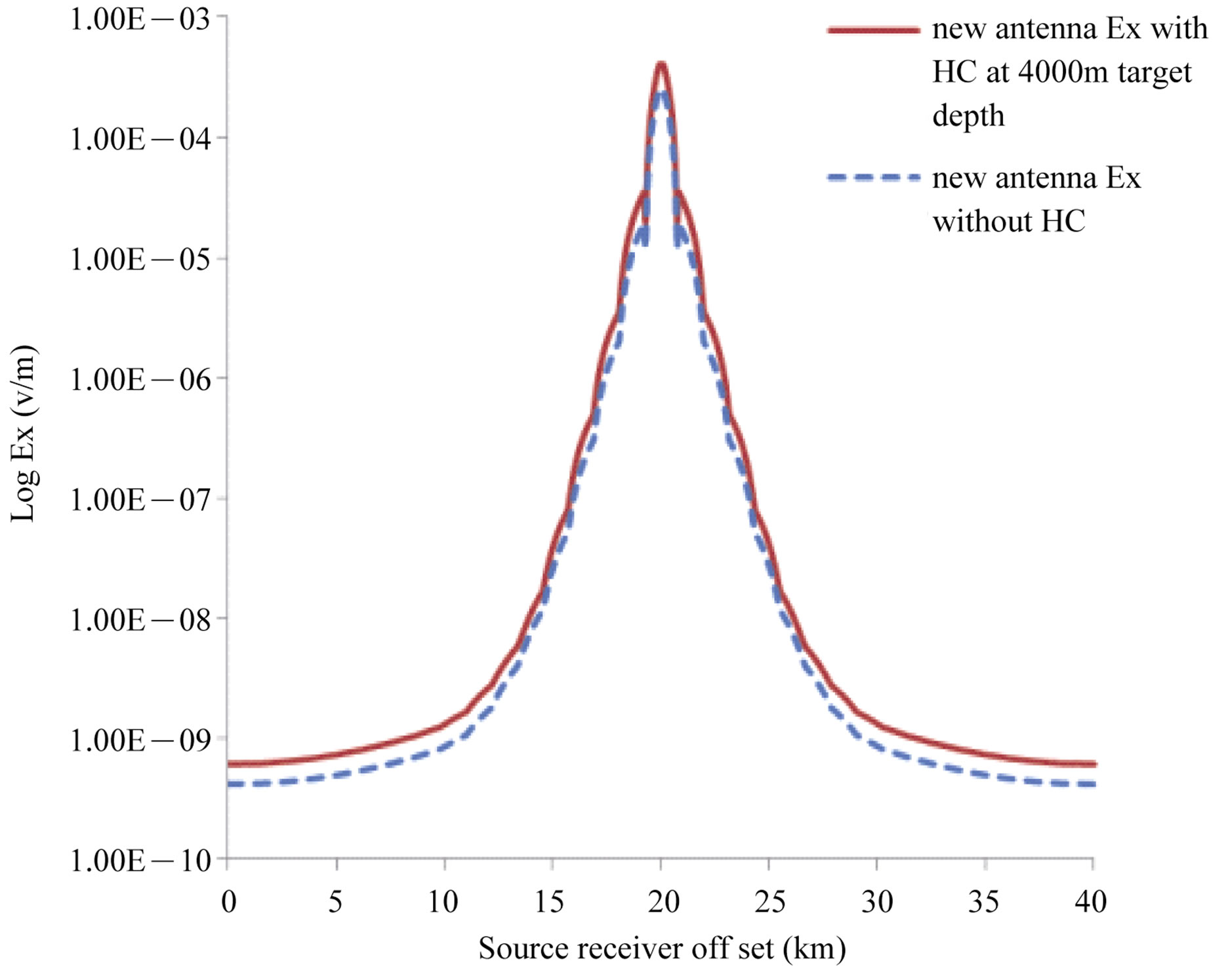 (h)
(h)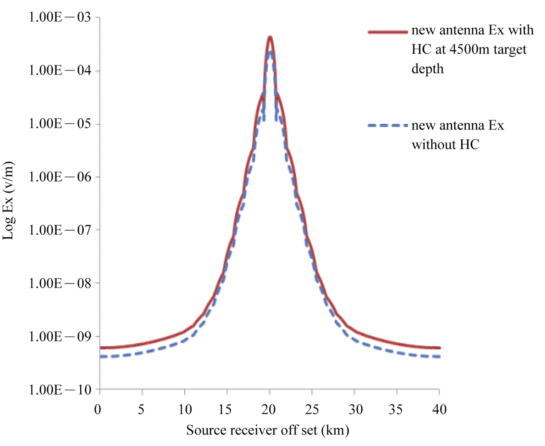 (i)
(i)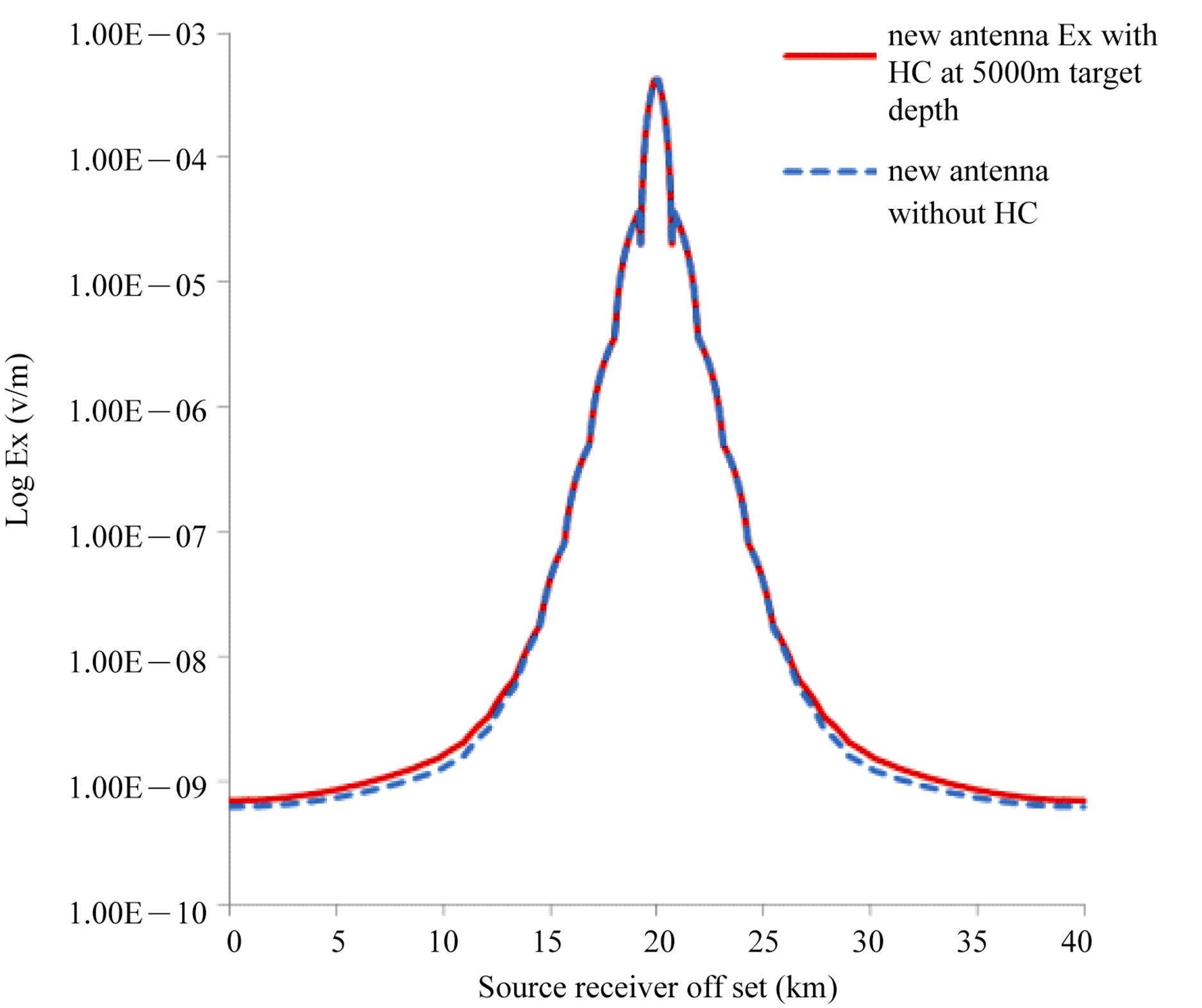 (j)
(j)
Figure 8. New antenna Ex-field MVO with different target positions (a) 500 m; (b) 1000 m; (c) 1500 m; (d) 2000 m; (e) 2500 m; (f) 3000 m; (g) 3500 m; (h) 4000 m; (i) 4500 m; (j) 5000 m.
new antenna shows 12% difference at 4250 m target depth in deep water and can be used to reduce the drilling risk factor for oil and gas industry until 4250 m target depth. Comparison of straight and new antenna is shown in Tables 3 and 4 respectively.
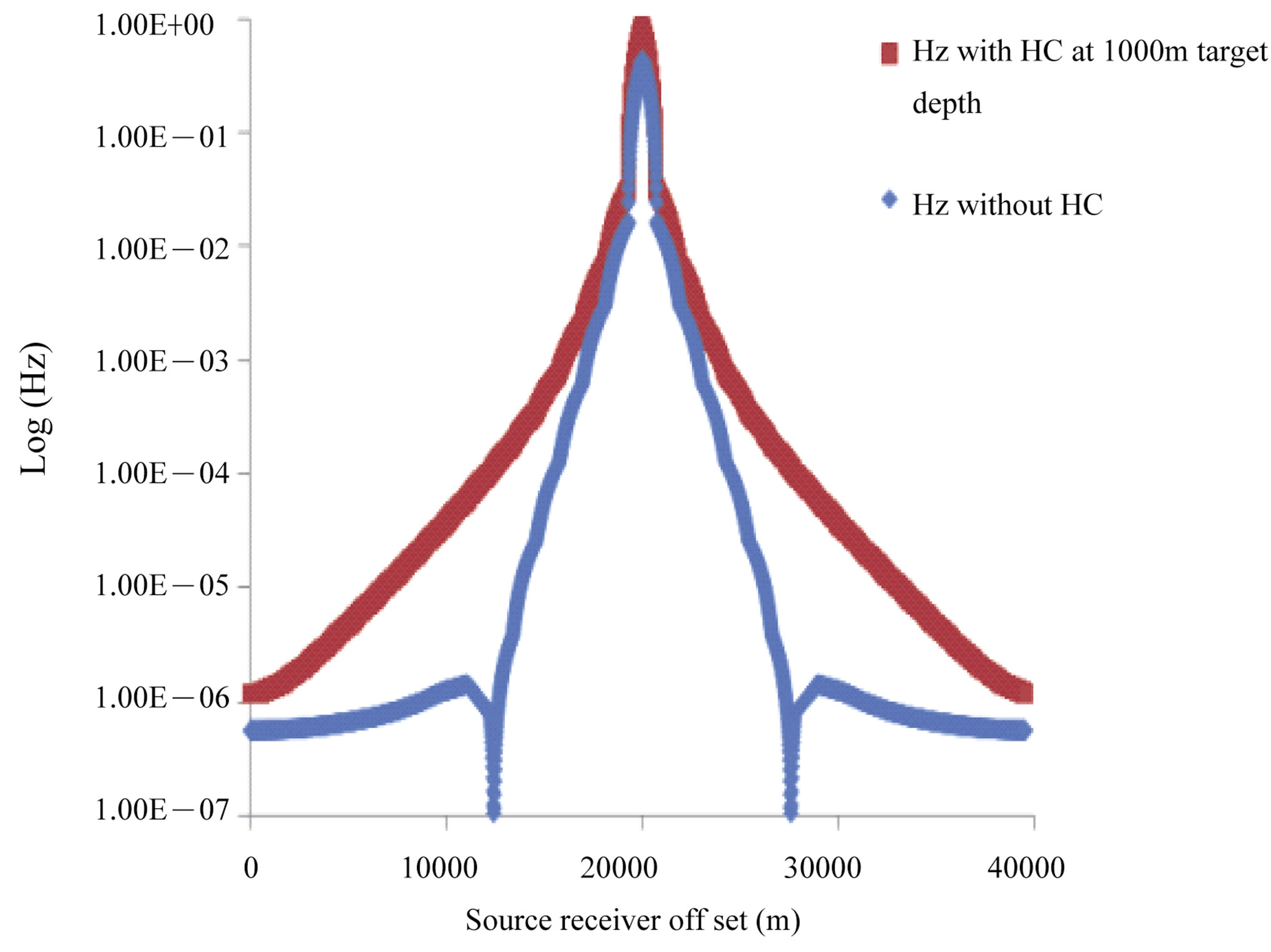
New antenna Hz magnitude verses offset comparison with different target depth is given Figure 9. Solid lines in MVO plot represent hydrocarbon response where as dotted lines without hydrocarbon reservoir. For near offset less than 3 km direct wave dominate and hydrocarbon reservoir presence cannot be predicted. Greater than 3km offset in deepwater guided response dominate the direct wave’s response. Due to this reason greater than 3 km offset can predict about the presence of hydrocarbon reservoir. At 500 m target depth new antenna shows 540% Hz field strength than without hydrocarbon reservoir. As the target depth increases the Hz field strength decreases due to the skin depth effect. At 4250 m target depth Ex response was 12% where as Hz 16% with new antenna design and Hz component able to delineate deep target better than Ex component. Analysis of new antenna results reveals that it can be used to detect deep target up to 4250 m target depth below the sea floor in deep water.
3.4. New Antenna Curvature Study with Different Target Depths
New antenna with different curvatures was simulated in CST software to know the maximum target depth this antenna can detect. Four different curvatures were used in this analysis. Electric and magnetic field response of four different curvatures is given (Table 5). From analysis it was observed that new antenna with curvature h = r/3 gave better electromagnetic field response as compared to other curvatures of this new antenna. Three different curvatures were used for 500 m target depth study to validate the best curvature for deep target for sea bed
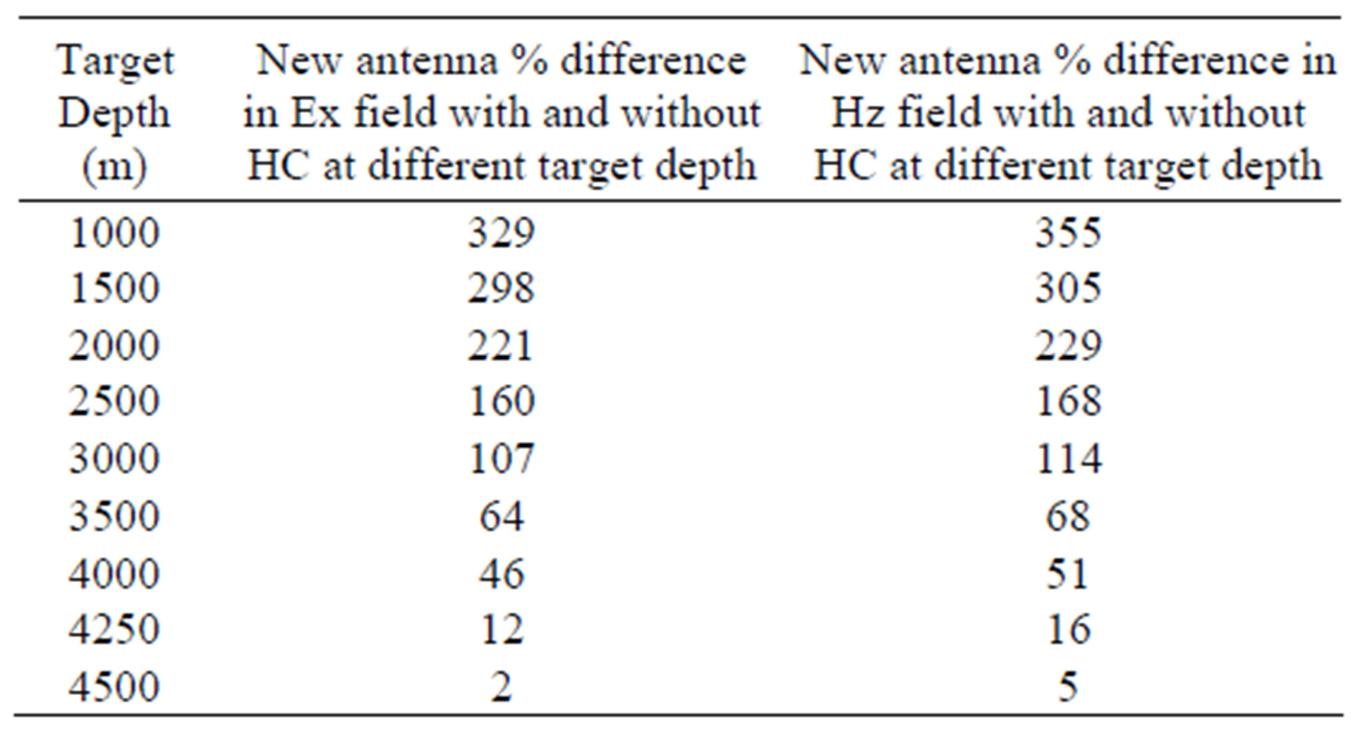
Table 3. Straight antenna Ex and Hz field response % difference comparison at different target depth with and without HC.
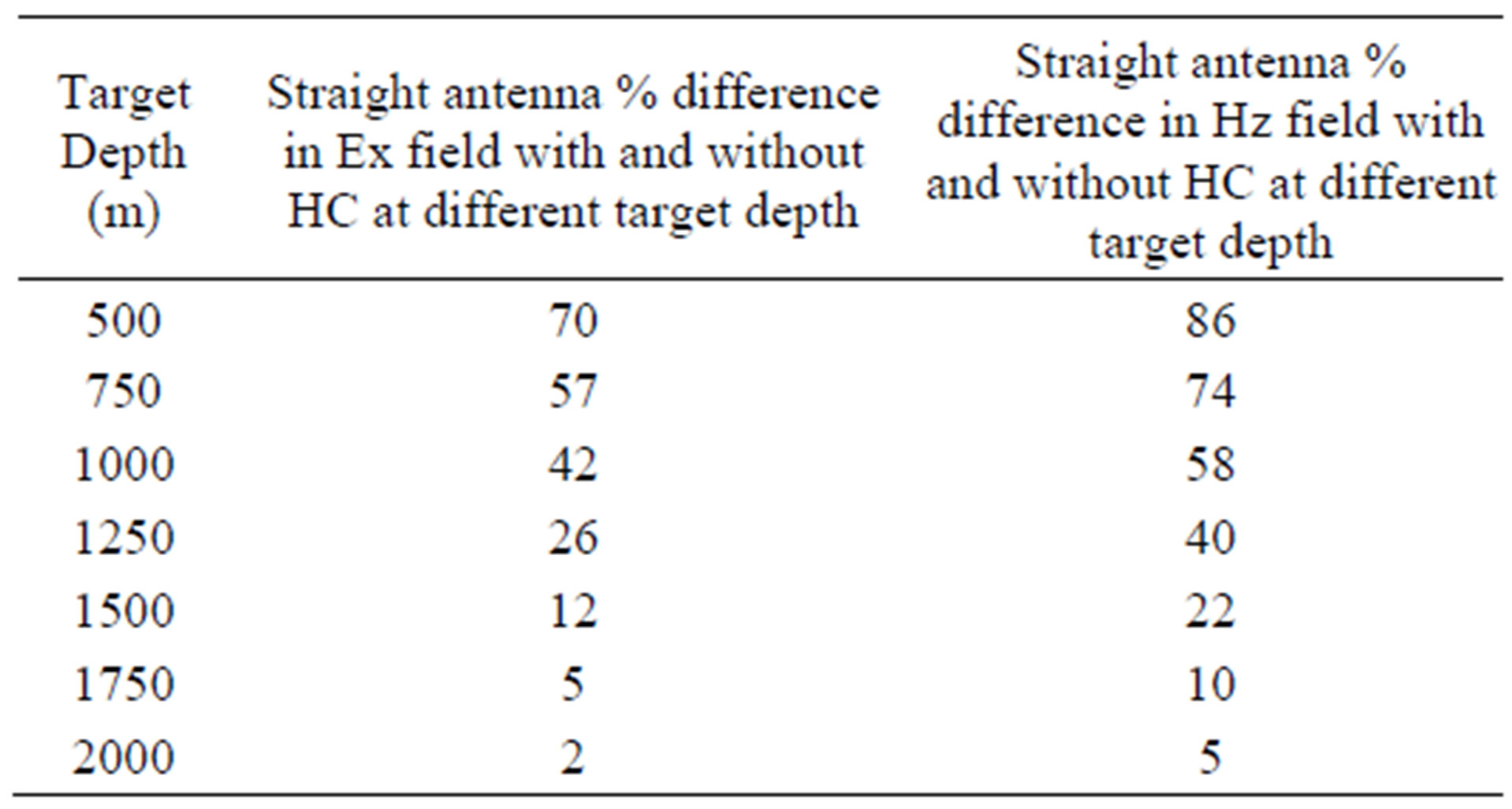
Table 4. New antenna Ex and Hz field response % difference comparison at different target depth with and without HC.
 (a)
(a)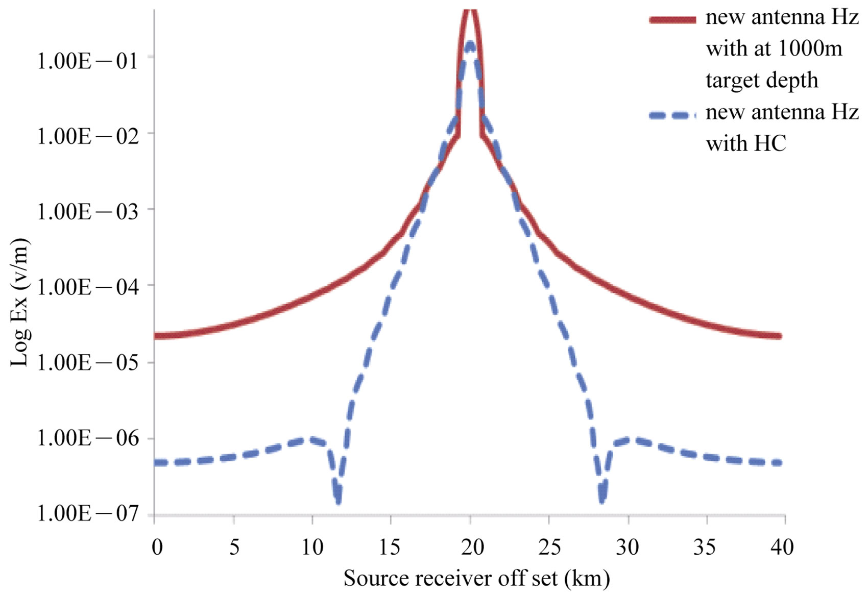 (b)
(b) (c)
(c)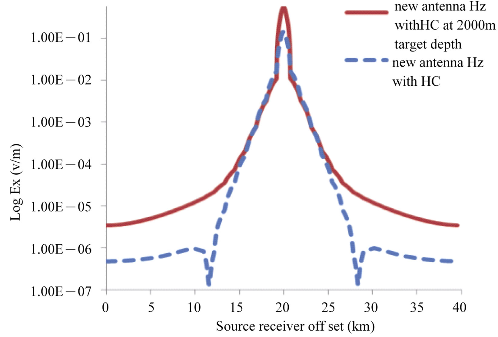 (d)
(d)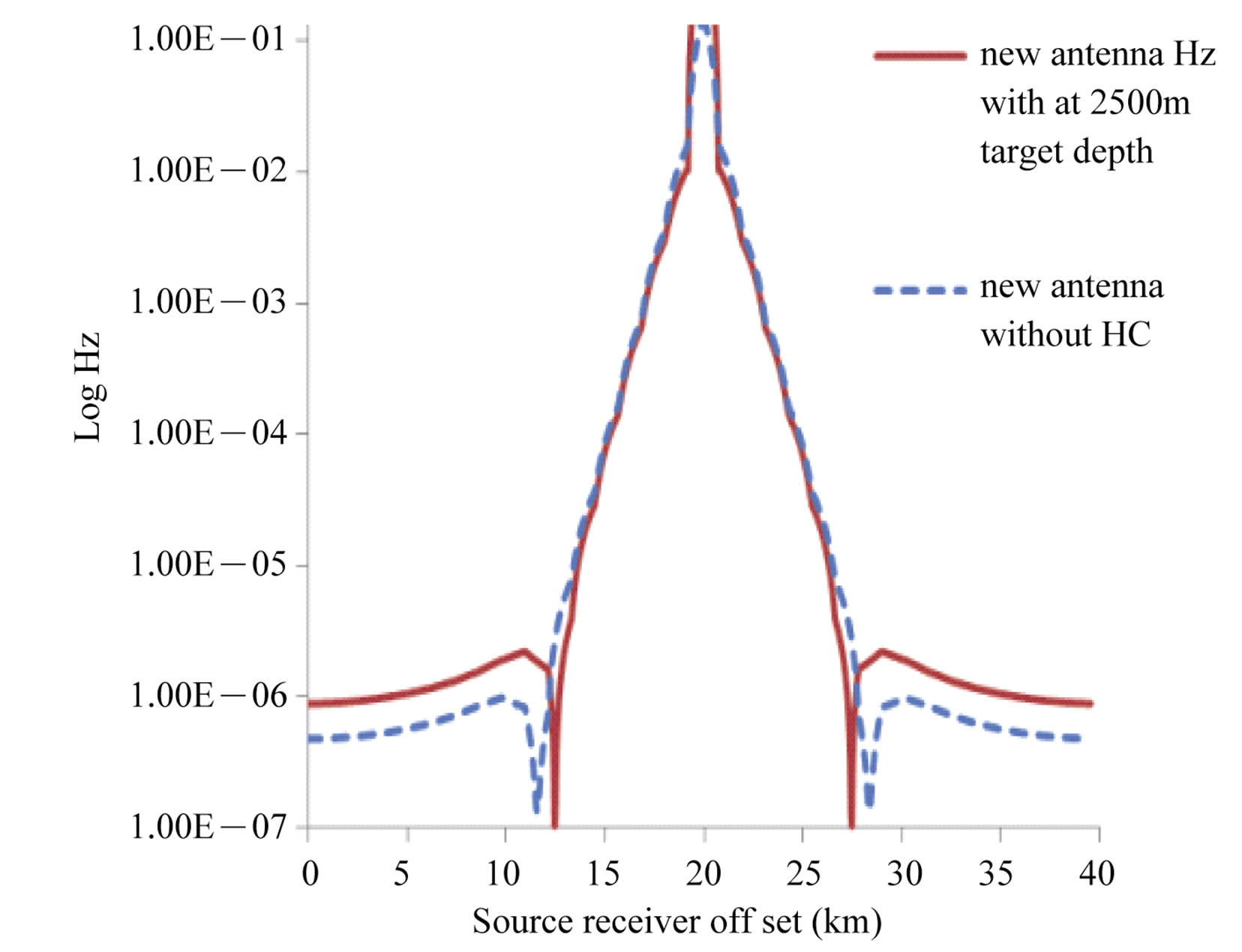 (e)
(e)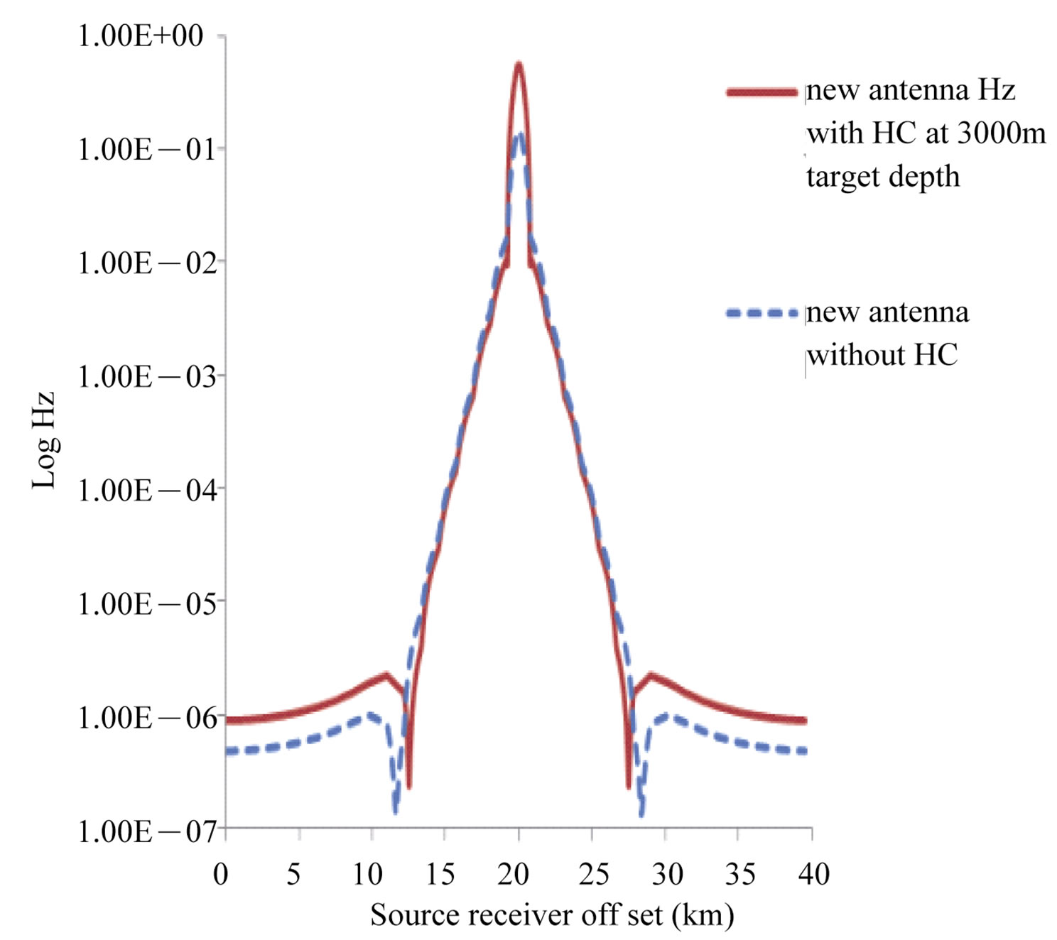 (f)
(f)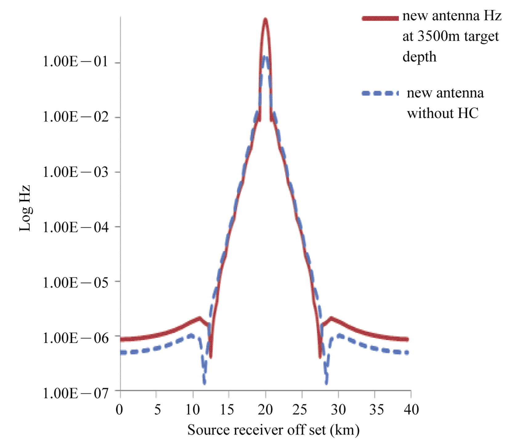 (g)
(g)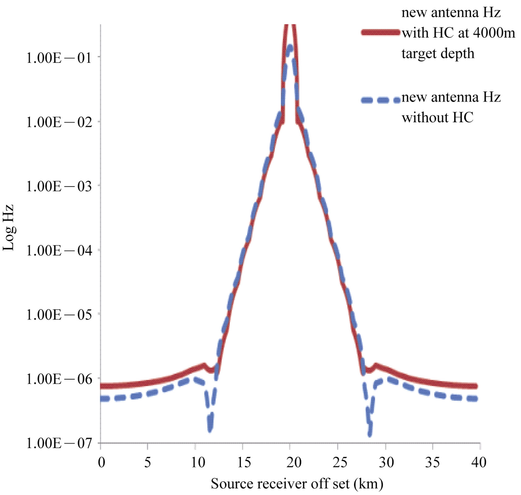 (h)
(h)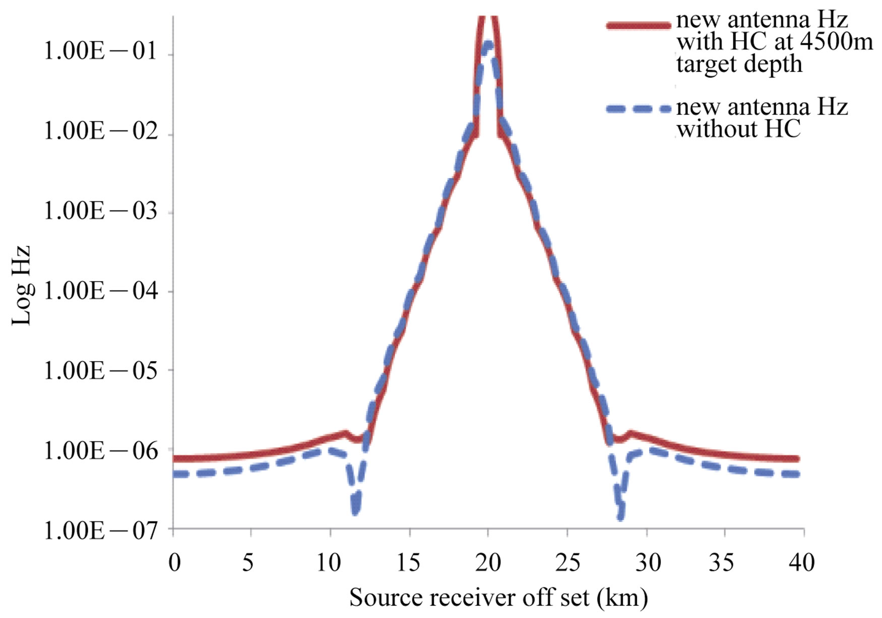 (i)
(i)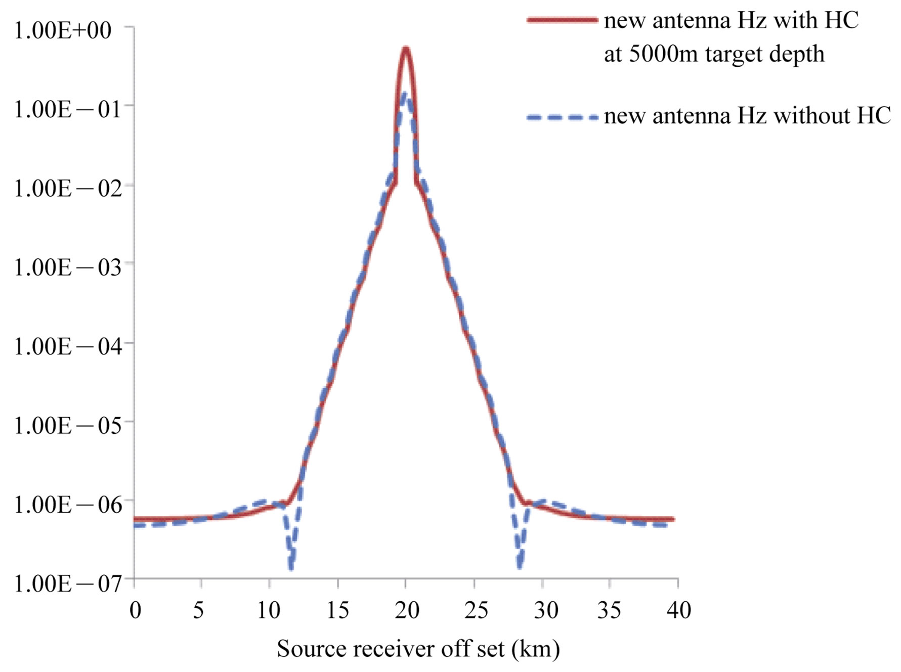 (j)
(j)
Figure 9. New antenna Hz-field MVO with different target positions (a) 500 m; (b) 1000 m; (c) 1500 m; (d) 2000 m; (e) 2500 m; (f) 3000 m; (g) 3500 m; (h) 4000 m; (i) 4500 m; (j) 5000 m.
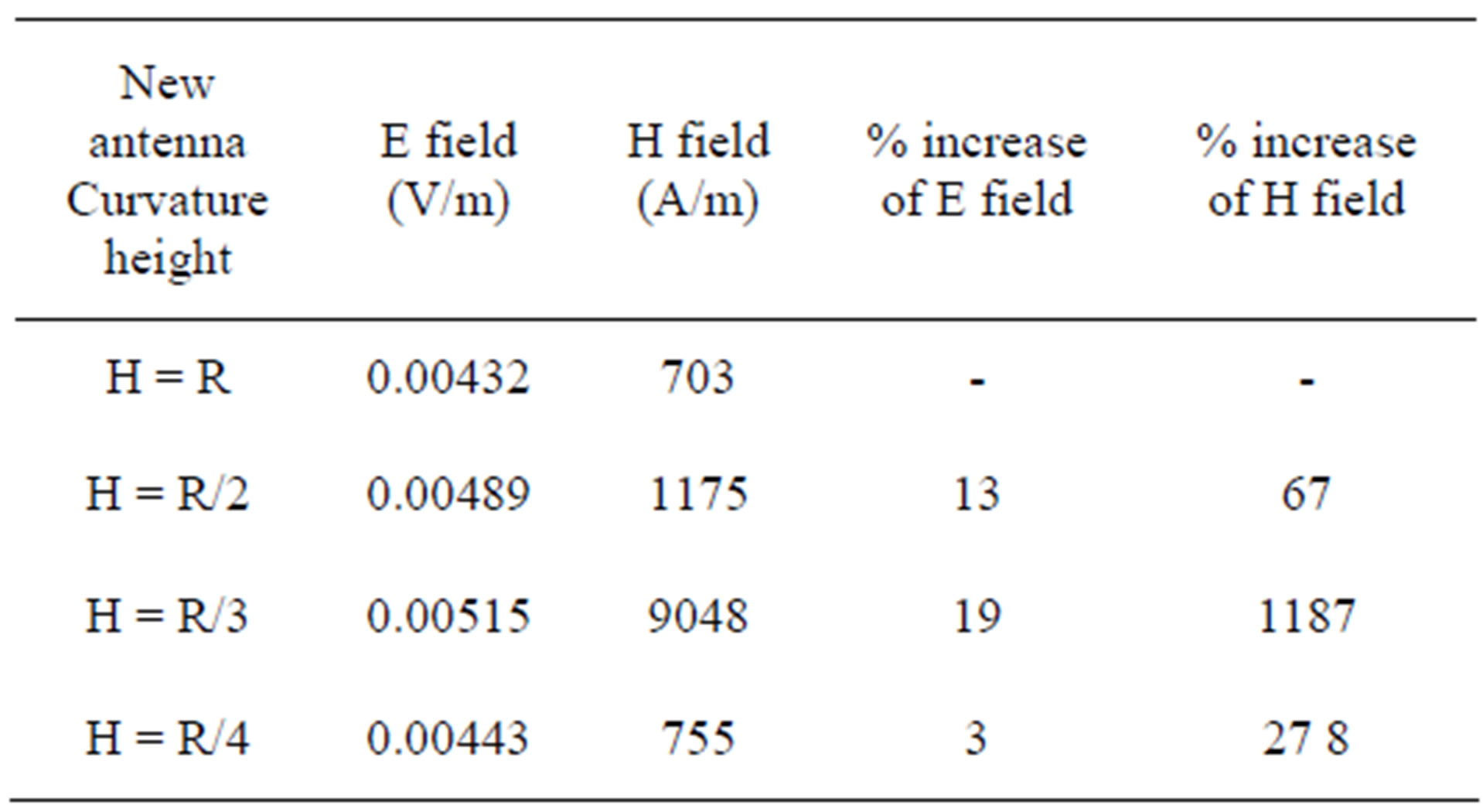
Table 5. New antenna Ex and Hz field response % difference comparison at different target depth with and without HC.
logging. Electric field response of new antenna different curvatures is given (Figure 10). As the attenuation factor for electromagnetic field strength for 500 m target depth is the same but the electromagnetic field strength for curvature h = r/3 is 1187% higher than other curvatures. Electromagnetic field response with hydrocarbon reservoir is given in (Figure 10). Log scale is used to plot the new antenna different curvatures electric field response to see the difference of electromagnetic field strength at 500 m target depth.
3.5. Numerical Model for Straight and New Antenna with Different Curvatures for Deep Target in Deep Water Environment
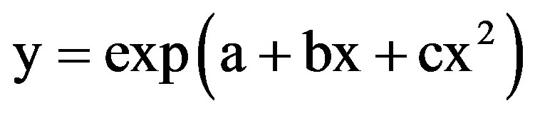
Numerical model is a very important to know the location hydrocarbon in sea bed logging. It can provide the information about the target depth at which target depth the electromagnetic wave signal provide information about hydrocarbon reservoir. Regression analysis was done for numerical model of electric field data at differrent target depths. Nonlinear regression technique is used to get the best fit mathematical function for input data. Simulated data for different target depth is used for numerical model for straight and new antenna data. Guided wave response data at different target depth is used for numerical model. Data fitting tool was used to fit the simulated data response. Equations for fitting data were obtained at different target depths. These equations were used for numerical model. Data fitting tool is used to fit the sea bed logging data for various target depths. Target depth 500 m to 1250 m target depth fitting of our proposed sea bed model data fitting is given Figure 10. Guided wave response is used for fitting the data. More than 800 data points are used for data fitting for survey area of 40 km × 40 km. General equation that best fit for electromagnetic field data is given (Equation (5)).
 (5)
(5)
In above equation y is the numerical model electric or magnetic field response, (a, b, c) are the constants where as x is the target depth. This general equation can be used to get the electric or magnetic field response at any target depth to locate the hydrocarbon reservoir.
Numerical model for straight antenna was plotted with the help of polynomial equation for different target depth. According to amperes law the electromagnetic field strength decreases with 1/r2 where r is the distance between source and receiver. Equation y = exp(a + bx + cx2) shows the electromagnetic field behavior with target depth where (a = –19.23, b = –1.41e–4, c = 1.57e–7) are constants x the target depth and y electric field response with corresponding target depth. Electromagnetic field strength decreases according to amperes law. Different target depths equations were plotted to get the numerical model and it was observed that straight antenna can detect up to 1.7 km target depth given Figure 11.
Numerical model for new antenna with curvature h = r was plotted with the help of polynomial equation for different target depth. Electric field response for each target depth was plotted to get the numerical model. Circles are the data with the change of target depth. Again data fitting tool was used to know the trend of this numerical model. General equation Y = exp(a + bx + cx2) shows the electromagnetic field behavior with target depth where (a = –17.01, b = –9.40E–4, c = 1.37E–8) are constants x the target depth and y electric field response with corresponding target depth. This general equation can be used
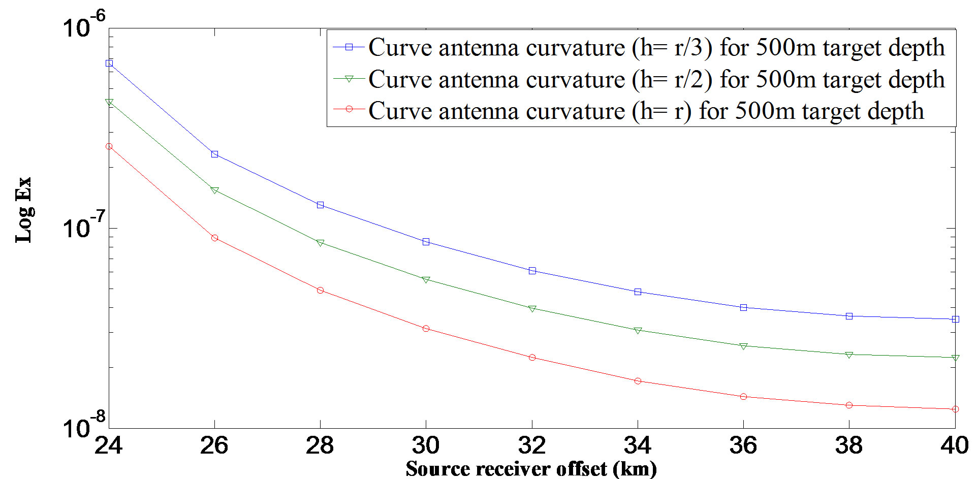
Figure 10. Different curvature study of new antenna at 500 m target depth.
to locate the hydrocarbon reservoir by putting the target depth only. According to amperes law the electromagnetic field strength decreases with 1/r2 where r is the distance between source and receiver. New antenna with this curvature can detect up to 3.5 km target depth is given Figure 12.
Numerical model for new antenna with curvature h = r/2 and h = r/3 was plotted with the help of polynomial equation for different target depths. Equation Y = exp(a + bx + cx2) shows the electromagnetic field behavior with target depth (a = –16.58, b = –7.03E–4, c = 6.47E-8) where as curvature h= r/3 (a = –16.24, b = –6.05E–4, c = 5.40E–8) are constants x the target depth and y electric field response with corresponding target depth. Electromagnetic field strength decreases according to amperes law. Change of curvature of this new antenna design has different focusing point and detects different target depths. Curvature h = r/2 detect up to 4 km target depth where as curvature h = r/3 can detect up to 4.5 km target depth is given (Figures 13-14) respectively. Numerical model (Equation (5)) was used to validate the electric field response for straight antenna and new antenna design for deep hydrocarbon target. At different target depths the electric field response from numerical model equation was within the range of electric field response as got from the simulated results. Straight and new antenna electric field response is given (Tables 6-7) respectively.
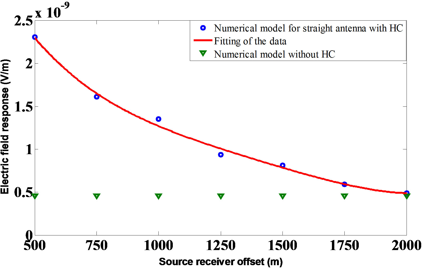
Figure 11. Numerical model with straight antenna used for sea bed logging.
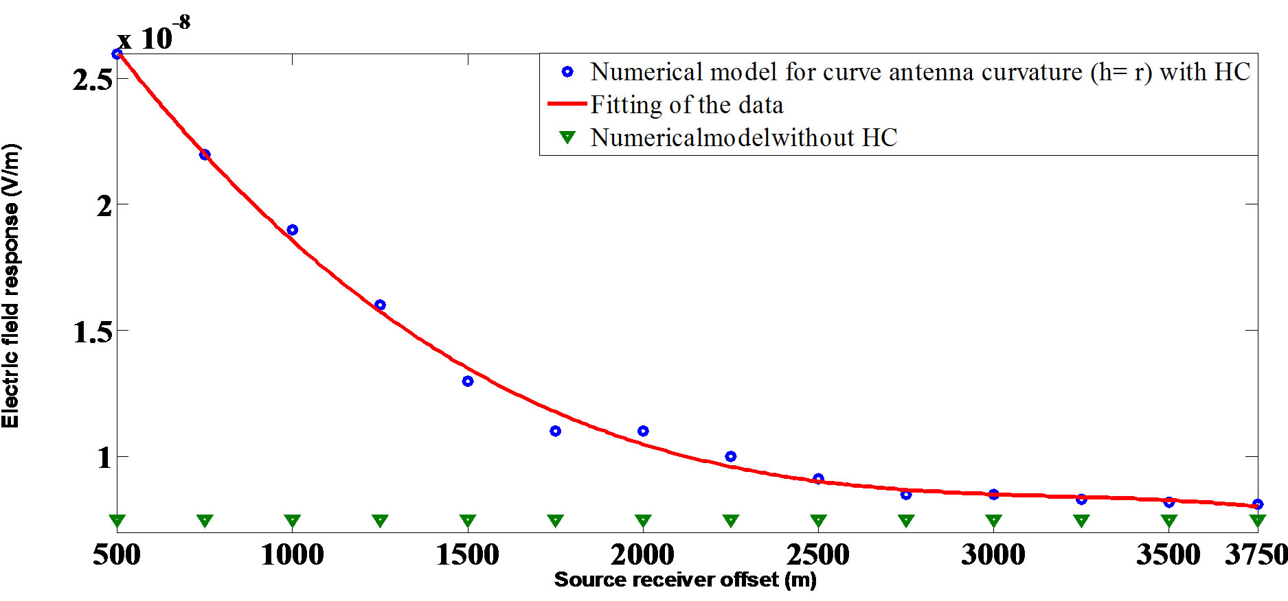
Figure 12. Numerical model with antenna curvature h = r with different target depth.
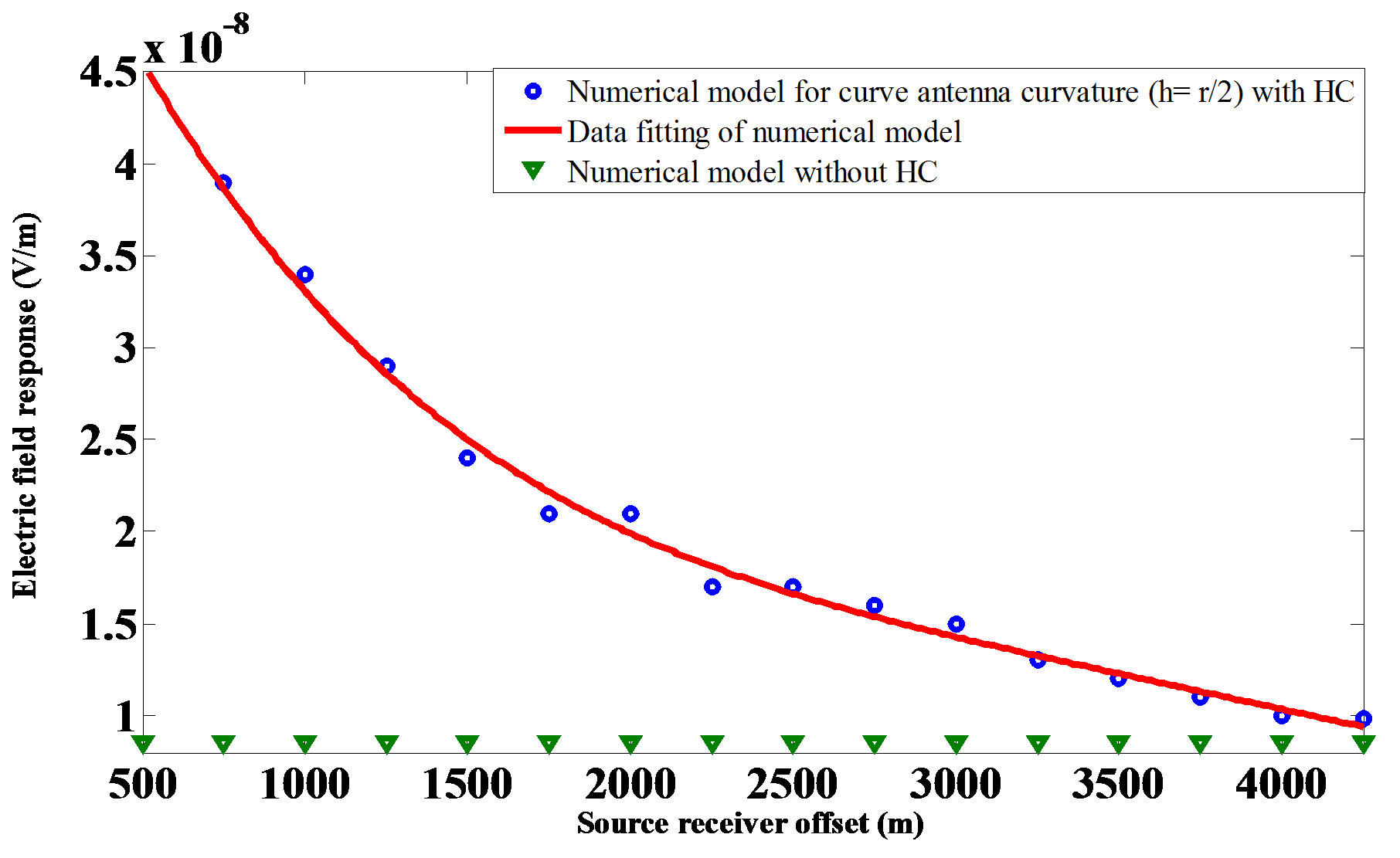
Figure 13. Numerical model with antenna curvature h = r/2 with different target depth.
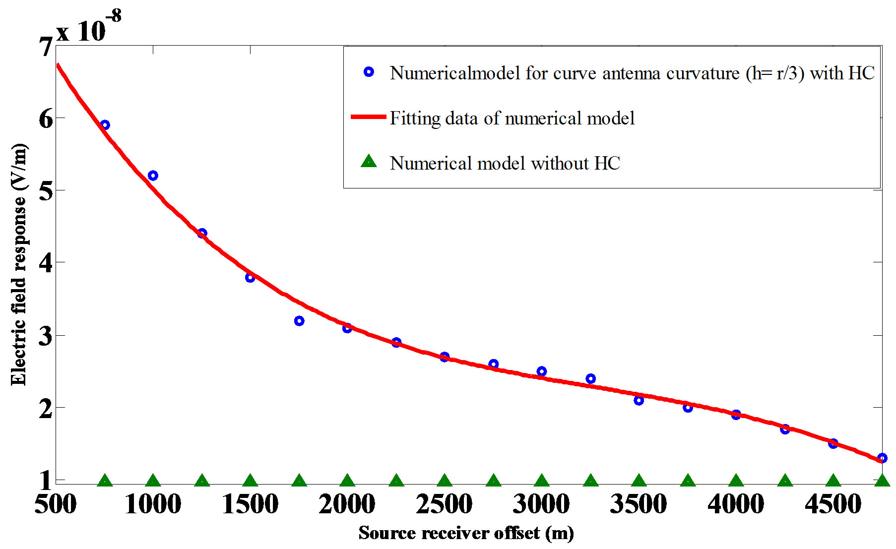
Figure 14. Numerical model with antenna curvature h = r/3 with different target depth.
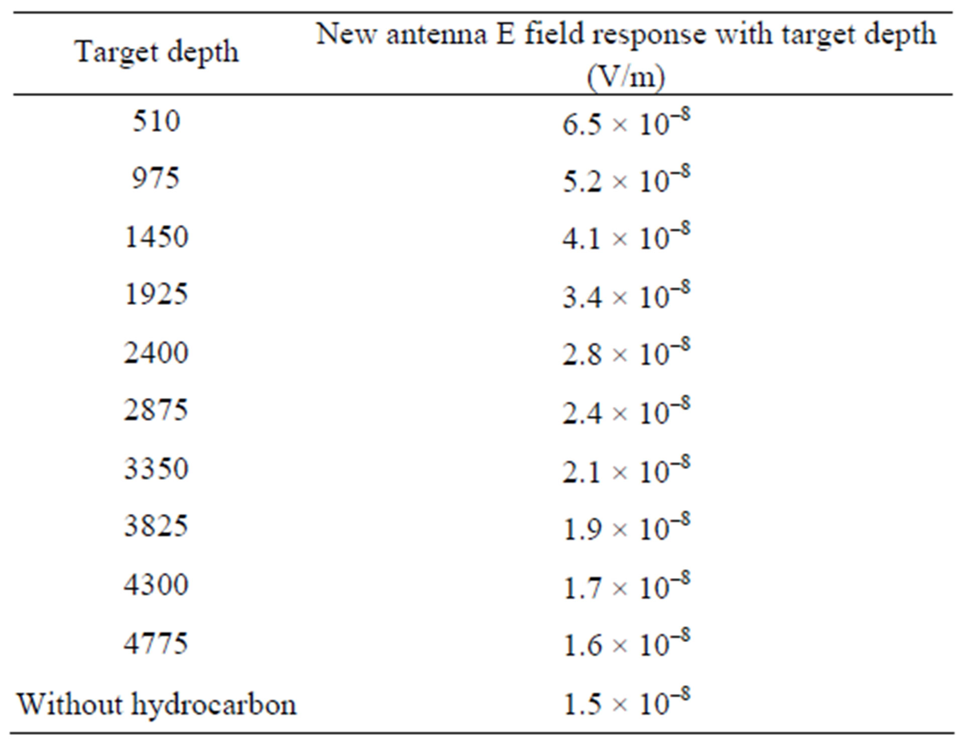
Table 6. Straight antenna E field response calculation at different target depth with the help of numerical model.
4. Conclusion
Electromagnetic field components response with hydrocarbon reservoir at 500 m target depth was done which shows that Ex and Hz components shows better delineation than other components. Ex field response for new antenna shows 329% resistivity contrast at target depth of 1000 m where as straight antenna showed 70% resis-
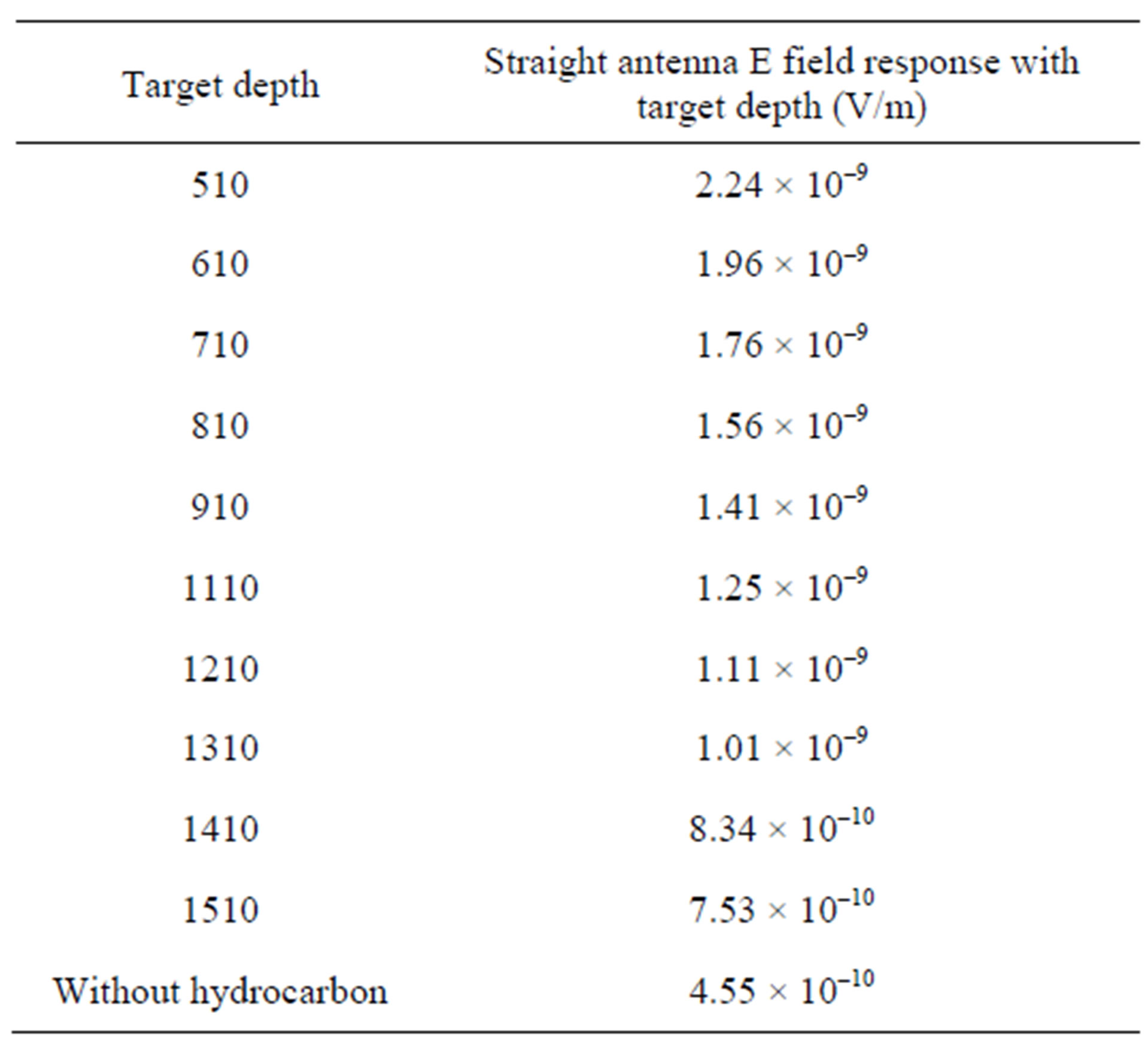
Table 7. New antenna E field response calculation at different target depth with the help of numerical model.
tivity contrast at same target depth. Hz field shows 355% resistivity contrast where as straight antenna shows 86%. From these results it was analyzed that Hz field shows better delineation for hydrocarbon detection. It was also observed that at frequency of 0.125 Hz, new antenna gave 46% better delineation of hydrocarbon at 4000 m target depth. Numerical modeling was done to know the exact target depth at which this new antenna can detect in deep water environment. It was observed that new antenna can detect 4.5 km target depth.
REFERENCES
- L. MacGregor and M. Sinha, “Use of Marine ControlledSource Electromagnetic Sounding for Sub-Basalt Exploration,” Geophysical Prospecting, Vol. 48, No. 6, 2000, pp. 1091-1106. doi:10.1046/j.1365-2478.2000.00227.x
- B. Tossman, D. Thayer and W. Swartz, “An Underwater Towed Electromagnetic Source for Geophysical Exploration,” IEEE Journal of Oceanic Engineering, Vol. 4, No. 3, 1979, pp. 84-89. doi:10.1109/JOE.1979.1145427
- S. Johansen, et al., “Subsurface Hydrocarbons Detected by Electromagnetic Sounding,” First Break, Vol. 23, No. 3, 2005, pp. 31-36.
- N. Yahya, M. N. Akhtar, N. Nasir, A. Shafie, M. S. Jabeli, and K. Koziol, “CNT Fibres/Aluminium-NiZnFe2O4 Based EM Transmitter for Improved Magnitude vs. Offset (MVO) in a Scaled Marine Environment,” Journal of Nanoscience and Nanotechnology, 2011, in press.
- N. Yahya, M. N. Akhtar, N. Nasir, H. Daud and M. Narahari, “Forward Modeling of Seabed Logging by Finite Integration (FI) and Finite Element (FE) Methods,” DSL, 2011, in press.
- N. Yahya, M. Kashif, H. Daud, H. M. Zaid, A. Shafie, N. Nasir and A. See, “Fabrication and Characterization of Y3.0-XLaXFe5O12—PVA Composite as EM Waves Detector,” International Journal of Basic & Applied Sciences, Vol. 9, No. 9, 2009, pp. 131-134.
- N. Nasir, N. Yahya, M. N. Akhtar, M. Kashif, A. Shafie, H. Daud and H. M. Zaid, “Magnitude Verses Offset Study with EM Transmitter in Different Resistive Medium,” Journal of Applied Sciences, Vol. 11, No. 7, 2011, pp. 1309-1314.
- M. N. Akhtar, N. Yahya, H. Daud, A. Shafie, H. M. Zaid, M. Kashif and N. Nasir, “Development of EM Wave Guide Amplifier Potentially Used for Seabed Logging,” Journal of Applied Sciences, Vol. 11, No. 7, 2011, pp. 1361-1365.
- M. Unsworth, “New Developments in Conventional Hydrocarbon Exploration with Electromagnetic Methods,” CSEG Recorder, 2005, pp. 34-38. http://www.ualberta.ca/~unsworth/papers/2005-CSEG-recorder-unsworth-apr05_07.pdf
- P. Clemmow, “The Theory of Electromagnetic Waves in a Simple Vanisotropic Medium,” Proceedings of the Institution of Electrical Engineers, Vol. 110, No. 1, 1963, pp. 101-106.
- F. N. Kong, H. Weterdahl, S. Ellingsrud, T. Eidesmo and S. Johansen, “A Possible Direct Hydrocarbon Indicator for Deep Sea Prospects Using EM Energy,” Oil and Gas Journal, Vol. 100, No. 19, 2002, pp. 30-38.
- C. S. Cox, S. C. Constable, A. D. Chave and S. C. Webb, “Controlled Source Electromagnetic Sounding of the Oceanic Lithosphere,” Nature, Vol. 320, 1986, pp. 52-54. doi:10.1038/320052a0
- M. C. Sinha, P. D. Patel, M. J. Unsworth, T. R. E. Owen and M. G. R. MacCormack, “An Active Source Electromagnetic Sounding System for Marine Use,” Marine Geophysical Research, Vol. 12, No. 1-2, 1990, pp. 59-68. doi:10.1007/BF00310563
- P. D. Young and C. S. Cox, “Electromagnetic Active Source Sounding Near the East Pacific Rise,” Geophysical Research Letters, Vol. 8, No. 10, 1981, pp. 1043-1046. doi:10.1029/GL008i010p01043
- E. Um and D. Alumbaugh, “On the Physics of the Marine Controlled-Source Electromagnetic Method,” Geophysics, Vol. 72, No. 2, 2007, pp. WA13-WA26.
- S. C. Webb, S. C. Constable, C. S. Cox and T. K. Deaton, “A Seafloor Electric Field Instrument,” Journal of Geomagnetism and Geoelectricity, Vol. 37, No. 12, 1985, pp. 1115-1129. doi:10.5636/jgg.37.1115
- A. D. Chave, S. C. Constable and R. N. Edwards, “Electrical Exploration Methods for the Seafloor Electromagnetic Methods in Applied Geophysics,” Electromagnetic Methods in Applied Geophysics, Vol. 2, 1992, pp. 931- 966.
- T. Eidesmo, S. Ellingsrud, L. M. MacGregor, S. C. Constable, M. C. Sinha, S. Johansen, F. N. Kong and H. Westerdahl, “SeaBed Logging (SBL), a New Method for Remote and Direct Identification of Hydrocarbon Filled Layers in Deepwater Areas Using Controlled Source Electromagnetic Sounding,” First Break, Vol. 20, No. 3, 2002, pp. 144-152.
- G. M. Hoversten, G. A. Newman, N. Geier and G. Flanagan, “3D Modeling of a Deepwater EM Exploration Survey,” Geophysics, Vol. 71, No. 5, 2009, pp. G239- G248.
- P. D. Aversana and M. Vivier, “Expanding the Frequency Spectrum in Marine CSEM Applications,” Geophysical Prospecting, Vol. 57, No. 4, 2008, pp. 573-590.
- B. Niels, L. Christensen and K. Dodds, “Special Section —Marine Controlled Source Electromagnetic Methods1D Inversion and Resolution Analysis of Marine CSEM Data,” Geophysics, Vol. 72, No. 2, 2007, pp. WA73- WA84. doi:10.2529/PIERS060822070325
- L. Gelius, “Multi-Component Processing of Sea Bed Logging Data,” Progress in Electromagnetic Research Online, Vol. 2, No. 6, 2006, pp. 589-593.
- A. Shaw, A. I. Al-Shamma’a, S. R. Wylie and D. Toal, “Experimental Investigations of Electromagnetic Wave Propagation in Seawater,” Proceedings of the 36th European Microwave Conference, Manchester, 10-15 September 2006, pp. 572-575.
- Y. Li and K. Key, “2D Marine Controlled Electromagnetic Modeling: An Adaptive Finite Element Algorithem,” Geophysics, Vol. 72, No. 2, 2007, pp. 51-62.
NOTES
*Corresponding author.