Journal of Electromagnetic Analysis and Applications
Vol. 3 No. 10 (2011) , Article ID: 8145 , 7 pages DOI:10.4236/jemaa.2011.310066
Finite Step Conjugate Gradients Methods for the Solution of an Impedance Operator Equation Arising in Electromagnetics*
![]()
Sys’com Laboratory, National Engineering School of Tunis (ENIT), Tunis, Tunisia.
Email: Haifa.belhadj@yahoo.fr, Taoufik.aguili@gmail.com
Received August 11th, 2011; revised September 10th, 2011; accepted September 23rd, 2011.
Keywords: Conjugate Gradient Method, Generalized Equivalent Circuit Method, MoM, Electromagnetic Computational, Scattering
ABSTRACT
A class of finite step iterative methods, conjugate gradients, for the solution of an operator equation, is presented on this paper to solve electromagnetic scattering. The method of generalized equivalent circuit is used to model the problem and then deduce an electromagnetic equation based on the impedance operator. Four versions of the conjugate gradient method are presented and numerical results for an iris structure are given, to illustrate convergence properties of each version. Computational efficiency of these methods has been compared to the moment method.
1. Introduction
One of the major problems in machine computation is to find an effective method to solve large system in reasonable time. There is, of course, no best method for all system because the goodness of a method depends to some extent upon the particular problem to be solved. Iterative methods have been considered to be more efficient for large system [1]. In fact, the preferred method is the one which insures rapid convergence after a finite number of steps, which has less numerical complexity and which in each steps should give information about the solution and should yield a new and better estimate than the previous one. The conjugate gradient [1,2] method is considered among the most efficient iterative scheme for the solution of a system of equations. In fact, with an arbitrary initial guess, methods of conjugate gradients converge to the solution in at most N iterations, where N is the problem dimension. This method requires much less storage than the conventional matrix methods for a problem with high complexity. In literature variants of this method are developed and used to solve electromagnetic problems [3-6].
In this paper, some comparison data are given to show convergence properties of 4 versions of the conjugate gradients methods comparing to the moment method (MoM) [7] and to show the rate of convergence of each algorithm. Each version of the CGM used here has been developed using the new implementation of the CG algorithm presented in previous work [8].
This paper is organized as follows: Section 2 presents the problem formulation; it briefly reminds the methodology to extract the equivalent circuit and deduce the equation to solve. Section 3 presents four versions of the conjugate gradients methods. These algorithms have been applied to solve the operator equation deducted from the equivalent circuit. Comparison data on CPU time and simulation results have been presented in section four in order to choose the most convenient algorithm for this type of problem. Last section draws conclusion.
2. Numerical Formulation of the Problem
Let consider the Cantor iris located in the cross section of a parallel-plates waveguide [8]. The aim is to compute the current density of the considered structure when illuminated by its fundamental mode: the TEM mode. The waveguide used is called EMEM waveguide, it is composed of two perfect electric walls to the top and the bottom, and lateral walls are magnetic. Boundary conditions are synthetically expressed by a Generalized Equivalent Circuit GEC method [9-11] which translates the relations between electric and magnetic fields into an equivalent circuit.
The equation, to solve, verified on the metallic part of the structure is given by:
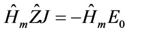 (1)
(1)
with  is an auto-adjoint operator,
  and
and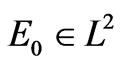 .
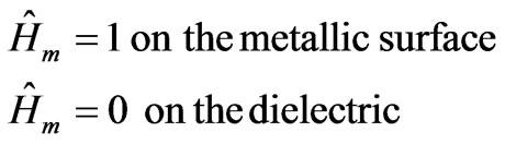
.  is the indicator of the metallic part of the discontinuity surface:
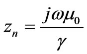
We remind that the impedance operator is given by the following formal relation [12]
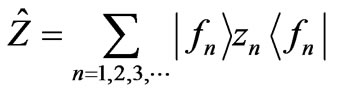 (2)
(2)
zn designs the impedance of each mode, and n is the mode number [12].
 (3)
(3)
where 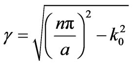 denotes the propagation constant and a designs the waveguide width among the x-axis.
The fn define the waveguide modal basis [11,12], and are determined as a function of the waveguide type.
Due to the invariance of the problem, only TEM mode and Transverse Electric modes exist. The mode basis is then given as following:
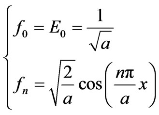 (4)
(4)
In this paper, we focus on solving the Equation (1) defined on the metallic part of the structure using variants of conjugate gradients methods.
The conjugate gradients methods have the same properties, all of them proceeds by generating successive approximations to the solution, and search directions used in updating iterates and residuals. Only a small number of vectors need to be kept in memory. Also the solution is improved at a steady rate throughout the iterative process.
In these algorithms, one has to evaluate the term . Some transformations are needed in order to compute this term. In fact, the impedance operator used here is described using modal basis, it is a discrete operator applied on the spectral domain. It is also called a spatial-spectral operator and it allows transition from spectral to spatial domain.
We remind that if we apply the impedance operator on J we obtain:
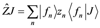 (5)
(5)
The x-axis is divided into N equivalent segments with negligible width and the current is assumed to be constant over each segment. The unknown function J is approximated by a linear combination of N independent pulse function with N unknowns coefficients J1, J2, ···, JN. The equation to solve on the metallic part of the structure, using variants of conjugate directions methods is given by:
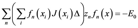 (6)
(6)
 is the uniform distance between any two sampling point xi and xi+1, it is equal to a/N and is called the cell density.
On the next section we present how can we solve such equation using variants of the CG algorithm.
3. Four Special Cases of the Conjugate Gradient Algorithm
The conjugate gradient method is special case of the conjugate direction method [1]. In this method the directions vector are selected to be mutually conjugate but have no further restrictions. Various formulas can be given, each leading to a special method.
We present four versions of the CG method, which yield simple algorithms, each of these variations has certain advantages [13].
3.1. The First Version
The first version of the CG presented here is used in literature for an Hermitian positive definite operator. In our case, we have a complex operator, but we are trying to apply this version to solve the Equation (6). The algorithm starts with an initial guess J0 of the unknown current. In all cases examined here a zero estimate is used. The initial residual and direction vectors are computed as following:

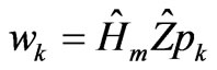
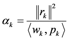
The following terms at the kth iteration are computed:
 ;
;
 ;
;
 ;
;
 ;
;
 ;
;
where pk is the direction vector and  is the scalar coefficient.
The values of the current obtained at the kth iteration are stored in the column vector Jk, with N components. Hence the ith element of J0 for example is the initial guess for the current over the ith segment.
The essential cost of this algorithm is the one of the operator vector product operation: .
.
The number of operation required at each step for this version of the CG method can be tabulated as Table 1.
Remind that the structure used is a regular iris on a rectangular waveguide. In the CG algorithm given above, it is observed that the initial residual and the term wk are multiplied by the Heaviside operator Hm, in order to impose the boundary conditions. So, each term evaluated here, contents numbers of zero equal to N/3, because the iris structure used is composed of three equivalent regions, two of them constitute the metallic part and the third one is the dielectric. The number of non zero elements is then equal to 2N/3. So, in Table 1, all the N operations needed for the computation of each term, should be changed by 2N/3, like is done in the computation of wk.
Note that, the computation of the term  is the most coasted operation in this algorithm. The computation of this term is equivalent to the computation of
  in Equations (5) and (6). This equation contains two series, so it needs 2N operations. Or, wk is equal to
 , so the coast of wk is then equal to 2(2N/3), and the number of operations is approximated by O(4N/3) per iteration. N is the number of unknown coefficients in the assumed current density expansion.
It is also observed that, one needs about O(N), storage locations to solve the present problem, utilizing this formulation rather than the conventional O(N2) for the matrix methods.
The total number of operations needed is then at about O(4pN/3), where p is the number of iterations.
3.2. The Second Version
This version of the CG is more general and is used for a not Hermitian operator [1,2]. In this work we are trying to use this algorithm in order to solve our operator equation.
The conjugate gradient algorithm for this case starts with a zero initial guess J0 and defines:
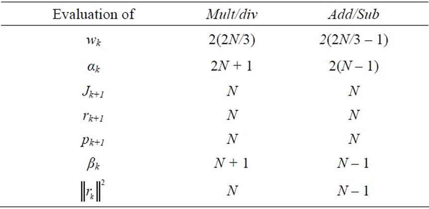
Table 1. The number of operations required at each equation in CGM.

And then develop each successive approximation by
 ;
;
 ;
;
 ;
;
 ;
;
 ;
;
where Z* is the adjoint operator of Z.
Comparing to the first version, an extra computations is required during the initial stage of the mentioned generalized CG algorithm. In this implementation, one has to do two operator/vector operations at each iteration, which increases the computation cost. It can be then concluded that the number of operation in the generalized CGM at each iteration is a little larger than O(4N/3).
3.3. The Third Version
Another version of this method is used also to a not Hermitian operator [1,2,13]. We adopted this algorithm to our electromagnetic problem in order to solve the same operator equation. The algorithm is given as


Iterate k = 1, 2,···


The third version’s implementation is very approached to the second one.
It is observed that the computational cost of this variant is particularly the same as the one needed in the second version.
3.4. The Forth Version: The BICG
The forth version tested here is the bi-conjugate gradient (BiCG) method. C.Lanczos [14] proposed early this algorithm in order to solve nonsymmetrical complex linear equation group. The bi-conjugate gradient for symmetrical complex linear equation group used in this work is described as follows:

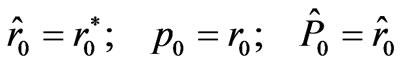
And then develop each successive approximation by
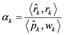


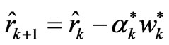


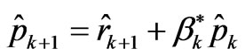
w* is conjugate of w, r* is conjugate vector of r, α* and β* are conjugate complex number of α and β.
The major advantages of the bi-conjugate gradient method over the generalized conjugate gradient method (version 2 and 3)for the solution of a symmetric complex linear equation group are, first, that the former requires only one matrixvector product whereas the latter requires two, and second, that the former converges much faster than the latter.
Remind that in all the versions described below, the indicator of the metallic part of the discontinuity surface of the structure , is introduced in the computation of the initial residual and the operator-vector products. Remind that this indicator is used to satisfy the boundary conditions, and to consider only the guide domain coincident with the metallic domain. This formulation is more economical on memory space and on computer cost. In fact, this version needs at about O(N) storage and O(4pN/3) operations, where p is the iterations number.
The stopping test used to decide about the convergence of these algorithms is the normalized squared residual error expressed as follow:
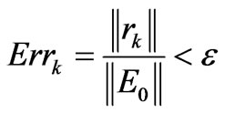
where ε is the accuracy fixed.
4. Numerical Convergence of the Conjugate Gradient Algorithms
As an example we consider the analysis of electromagnetic scattering from the Cantor iris in a parallel plate EMEM waveguide. The unknown current distribution over the metallic surface has been determinate using the various CG algorithms. The total and scattered electric fields have been then deducted.
4.1. Comparison between the Different Methods
All the forth versions tested in this work converge after a finite number of steps. We are interesting to the rate of convergence of these algorithms and have been compared to the one of the generalized Moment method. For the MoM the piecewise linear functions [15] are used as test functions. Results obtained, showing convergence rate, have been draped in Table 2. For the CG methods the stopping criterion was the normalized residual error which must be less than 10–7. Results are obtained with Intel core2duo 1.66G CPU and 2G-memory computer. All programs use matlabr2008a compiled language.
Numerical results are presented on the table below, for 3000 modes number. We are varying the number of unknowns to evaluate performance of each CG version. For the MoM the number of unknowns (N) designs the weighting functions number.
It is observed that the class of conjugate gradient methods has a better performance than the MoM. In fact, all the CG versions tested here converge faster than the MoM. That is explained by the fact that the CG methods needs less storage and less operations number than the MoM. It is also noted that the cputime is increasing as a function of the unknowns’ number.
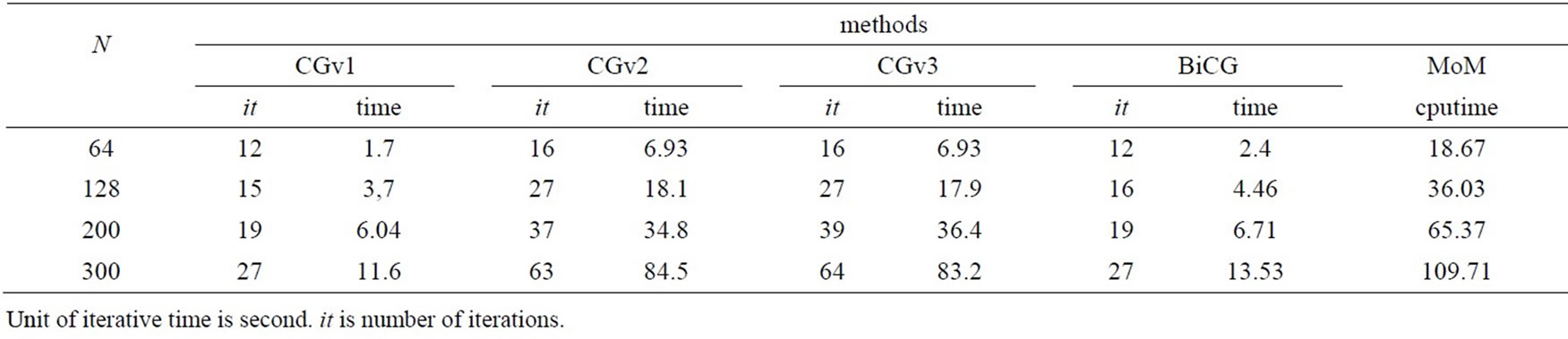
Table 2. Results of different methods (ε = 10–8).
Table 2 clearly illustrates that the BiCG and CGv1 are suitable for this type of problem as they are the faster methods. The BICG method is known as the most appropriate method to solve complex problem, which is the case of our operator.
The CGv1 is also recommended, as it needs less cputime than methods 2 and 3. But this method, known as the method of Hestenes, is used for an hermitian operator. In our case, we have a complex operator, but this method performs even well and is recommended. This shows the efficiency of these new CGs implementations.
The use of versions 2 and 3 for the solution of an arbitrary operator equation is in literature, recommended [13].
In our case, these algorithms converge faster than the MoM and slower than the CGv1 and the BiCG.
From a numerical standpoint, it appears both versions perform equally well, the cputime taken by both techniques is almost the same.
From Table 2, it can be also noticed that the convergence of the CGM is related to parameters such as the cell density used within the discretization.
Figure 1 shows the residual error behavior for the BiCG and the CG version 2 and 3 as a function of the iterations number.
It is observed, that all versions converged in a small number of steps. The number of iterations needed to reach convergence is far less than the problem dimension, which shows the efficiency of this formulation. So, the total number of operations needed, is proportional to pN, and is far less than N3 for the conventional matrix methods.
Figure 1 shows that, methods 2 and 3 both converged to a good solution (ε < 10–4) in 21 iterations, even though the initial guess was taken to be zero. For the second version magnitudes of the residuals decrease monotonically at each iteration. For the third version, even though the error between the true solution and the solution at the end of iteration decreases, the residual is increasing and decreasing randomly, it do not go down until the end. For the BiCG the residual is decreasing monotonically and fastly, which makes this version more adequate for this type of problem.
4.2. Simulation Results
After one obtains the induced electric current Jy numerically over the metallic surface, with a given excitation E0, using the CG algorithm, other parameters, such as the scattered and the total electric fields can be easily deducted.
The scattered field is computed by:
 (7)
(7)
Figure 2 presents the scattered electric field determined by each version.
It has been observed that from a theoretical standpoint, all the fourth method performs equally well. Numerical simulation shows that results obtained using these methods are perfectly the same.
The total electric field is also represented and compared to the MoM.
The total electric field is computed by:
 (8)
(8)
Figure 3 draws the normalized total electric field
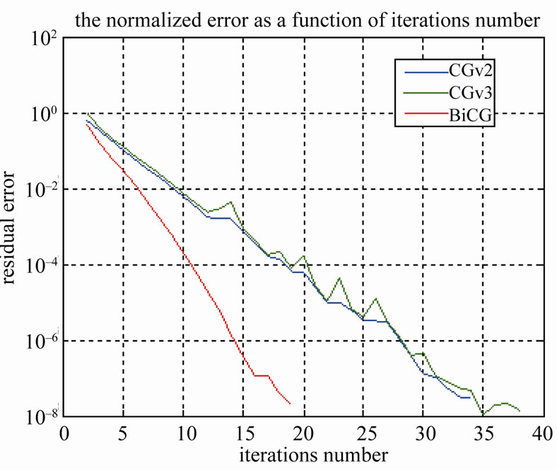
Figure 1. Errors of the three versions of the conjugate gradient method.
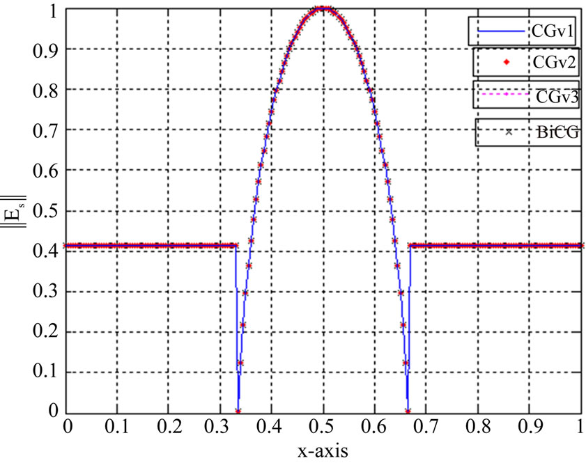
Figure 2. The normalized scattered electric field evaluated by the CG methods, with a = 22.9 mm at F = 2 Ghz (case of an EMEM waveguide), N = 200, n = 3000.

Figure 3. The normalized electric field depicted by the CGMs adopted in this work and the one evaluated by the MoM method.
evaluated by the conjugate gradients methods and the one computed by the moment method for the iris structure with EMEM walls.
For the moment method, results are plotted for 3000 sinusoidal mode functions; the piecewise test functions used are 200.
Figure 3 shows that the electric field behavior is with respect to the boundary conditions. It is also observed that results found at convergence by the CGM and the BiCG are conforming to the one found by the MoM.
In this section, it has been noticed that the class of CG methods as implemented, required less storage and less computational time than the MoM. Also simulation results obtained by each method are in obvious agreement.
5. Conclusions
In this paper, four versions of the CG algorithm are tested. These versions are applied to solve an operator equation arising in electromagnetic scattering. These converge to the solution in a finite number of steps starting from a zero initial guess. A numerical example is given to illustrate some properties of these versions.
It is observed that the CG methods appear more attractive than the conventional moment method as the error at each step is known and it provide less computational time. Also, CG methods require less storage.
Out of the four CG algorithms, the conjugate gradient version used for an Hermitian operator and the biconjugate gradient are recommended as they provide the lower computational time.
Solution obtained using the four versions is the same and a less residual is achieved.
Although, the first method is recommended for a Hermitian positive operator, it gives the better result when applying to our complex operator. This shows the efficiency of this implementation of the CG algorithm, which converges in all cases independently of the type of the operator used.
REFERENCES
- M. R. Hestenes and E. Stiefel, “Methods of Conjugate Gradients for Solving Linear Systems,” Journal of Research of the National Bureau of Standards, Vol. 49, No. 6, 1952, pp. 409-436.
- T. K. Sarkar, “The Conjugate Gradient Method as Applied to Electromagnetic Field Problems,” IEEE Antennas and Propagation Society Newsletter, Vol. 28, No. 4, 1986, pp. 4-14.
- A. F. Peterson and R. Mittra, “Convergence of the ConjuGate Gradient Method When Applied to Matrix Equations Representing Electromagnetic Scattering Problems,” IEEE Transactions on Antennas and Propagation, Vol. 34, No. 12, 1986, pp. 1447-1454. doi:10.1109/TAP.1986.1143780
- K. Barkeshli and J. L. Volakis, “Improving the ConvergeNce Rate of the Conjugate Gradient FFT Using Subdomain Basis Functions,” IEEE Transactions on Antennas and Propagation, Vol. 37, No. 7, 1989, pp. 893-900. doi:10.1109/8.29384
- T. A. Cwik and R. Mittra, “Scattering from a Periodic Array of Free-Standing Arbitrarily Shaped Perfectly Conducting or Resistive Patches,” IEEE Transactions on Antennas and Propagation, Vol. 35, No. 11, 1987, pp. 1226- 1234. doi:10.1109/TAP.1987.1143999
- T. K. Sarkar, E. Arvas and S. M. Rao, “Application of FFT and the Conjugate Gradient Method for the Solution of Electromagnetic Radiation from Electrically Large and Small Conducting Bodies,” IEEE Transactions on Antennas and Propagation, Vol. 34, No. 5, 1986, pp. 635- 640. doi:10.1109/TAP.1986.1143871
- R. F. Harrington and T. K. Sarkar, “Boundary Elements and the Method of Moments,” 5th International Conference of Boundary Elements, Hiroshima, 8-11 November 1983, pp. 31-40.
- H. Belhadj, S. Mili and T. Aguili, “New Implementation of the Conjugate Gradient Based on the Impedance Operator to Analyze Electromagnetic Scattering,” Progress in Electromagnetic Research B, Vol. 27, 2011, pp. 21-36.
- H. Baudrand, “Representation by Equivalent Circuit of the Integrals Methods in Microwave Passive Elements,” European Microwave Conference, Budapest, 10-13 September 1990, Vol. 2, pp. 1359-1364.
- T. Aguili, “Modélisation des Composantes SFH Planaires par la Méthode des Circuits Équivalents Généralisés,” Ph.D. Thesis, National Engineering School of Tunis, Tunis, 2000.
- H. Baudrand and D. Bajon, “Equivalent Circuit Representation for Integral Formulations of Electromagnetic Problems,” International Journal of Numerical Modelling Electronic Networks Devices and Fields, Vol. 15, No. 1, 2002, pp. 23-57. doi:10.1002/jnm.430
- H. Aubert and H. Baudrand, “L’Electromagnétisme par les Schémas Equivalents, ” in Français, Cepaduès, 2003.
- T. K. Sarkar and E. Arvas, “On a Class of Finite Step Iterative Methods (Conjugate Directions) for the Solution of an Operator Equation Arising in Electromagnetics,” IEEE Antennas and Propagation, Vol. 33, No. 10, 1985, pp. 1058-1066.
- C. Lanczos, “Solution of Systems of Linear Equtions by Minimized Iterations,” Journal of Research of the National Bureau of Standards, Vol. 49, 1952, pp. 33-53.
- D. R. Wilton and C. M. Butler, “Efficient Numerical Techniques for Solving Pocklington’s Equation and Their Relationship to Other Methods”, IEEE Transactions on Antennas and Propagation, Vol. 24, No. 1, 1976, pp. 83- 86. doi:10.1109/TAP.1976.1141286
NOTES
*Four versions of the CG method are presented in this paper and numerical results are given to compare computational efficiency of each version.