Journal of Electromagnetic Analysis and Applications
Vol. 3 No. 6 (2011) , Article ID: 5352 , 9 pages DOI:10.4236/jemaa.2011.36033
Lateral Waves near the Surface of Sea
![]()
1Department of Mathematics, Faculty of Science, Kafer El-Sheikh University, Kafer El-Sheikh, Egypt; 2Department of Mathematics, Faculty of Science, Ain Shams University, Abbassia, Cairo, Egypt; 3Department of Mathematics, Faculty of Science, Tanta University, Tanta, Egypt.
Email: {aboseida, stbishay, km_morabie}yahoo.com
Received February 25th, 2011; revised April 14th, 2011; accepted May 8th, 2011.
Keywords: Stratified Media, Rough Surface, Radiation in Sea, Lateral Waves
ABSTRACT
In this research, we investigate the propagation of lateral electromagnetic wave near the surface of sea. Interference patterns generated by the superposition of the lateral and direct waves along the sea surface (flat and rough) are shown. The field generated by a vertical magnetic dipole embedded below the sea surface (having a flat and perturbed upper surface) is shown to consist of a lateral-wave and a reflected-wave. Closed-form expressions for the lateral waves near the surface of the sea are obtained and compared with those mentioned for the reflected waves numerically for the considered model.
1. Introduction
Lateral electromagnetic waves generated by a vertical electric or magnetic dipole near the plane boundary between two different media like air and earth or air and sea have been the subject of investigation for many years beginning with the work of Sommerfeld. King [1] derived simple formulas for the transient field generated by a vertical electric dipole on the boundary between two dielectric half-space when the permittivity of one of these is much greater than that of the other. The roughness of the upper surface of the sea is considered by Bishay [2,3] to indicate the effect of the rough surface on the electromagnetic fields. Recently, Abo-Seida et al. [4] calculated the far-field radiated from a vertical magnetic dipole in sea with a rough upper surface. Besides, in previous studies [4], the Hankel transformations are estimated by using new technique developed by Long et al. [5] and Chew [6].
The present study is a further contribution to [4], so the Hankel transformations which were estimated by Abo-Seida et al. [4] are employed here. The previous studies [2,3] have obtained the formulas of the reflected waves in the region of the seawater, due to a vertical magnetic dipole in a three-layered conducting media by resolving the problem using the residue and saddle-point methods.
However, these methods, involve lengthy algebra and several transformations, which are very tedious and complicated. The new technique utilized in [4] was used in this study in order to obtain closed-form expressions of the lateral waves.
Firstly the form solutions of the far-field, due to a vertical magnetic dipole in a sea (three-layered conducting media) with variable interface are expanded as an infinite series. Then with the aid of the complex image theory [7], closed-form expression of the lateral waves near the sea surface due to the dipole are obtained. Besides, the physical meaning of the results is presented.
2. Geometrical Structure
We shall adopt the following model as illustrated in Figure 1. A small loop antenna, whose magnetic moment is , is located in the middle layer (i.e. in the sea) at depth
 , horizontally. An observing point
  is also located in the sea at depth
 . We suppose that the thickness of the sea is a, and that air is infinite upward and the ground downward along the z-axis. The groundsea interface is taken to be planar, while the air-sea interface varies slightly from its mean value, as shown in the figure. r is the distance between the source and the observing point P, and
  is that between P and the image of the source in the air.
The material constants are assumed to be as follows. The dielectric constant in the air, sea, and ground are  and
and , respectively. The magnetic permeability is taken equal to that of the free space in every layer. The

Figure 1. Geometrical configuration of the problem.
conductivity of the seawater and ground are  and
and , respectively.
3. The Lateral Waves in Sea
Lateral waves are the electromagnetic waves which are generated by vertical or horizontal dipoles on/or near the plane boundary between two electrically different media like air and earth or air and sea or ocean water. However, the lateral wave propagates from the antenna to the surface suffering some attenuation, then propagates in the air without attenuation over a long distance and then arrives at the receiver. Thus the communication is only through the lateral wave, since the direct and reflected waves are almost completely attenuated in the medium as in this case of flat upper surface.
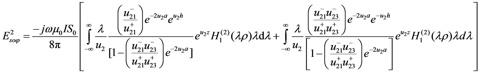
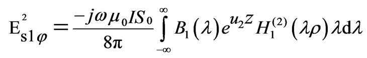
To evaluate the lateral waves, we return to the Equation (29) in [4] as

where ,
,  and its real part is positive,
  is the propagation constant of the medium under consideration.
 ,
,  and
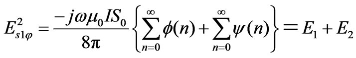
and  is the second-kind Hankel functions of order one. Therefore, we can write
  as
as
 (1)
(1)
where
 (2)
(2)
 (3)
(3)
According to the complex image theory [7], when condition  is satisfied, we have
 ,
,
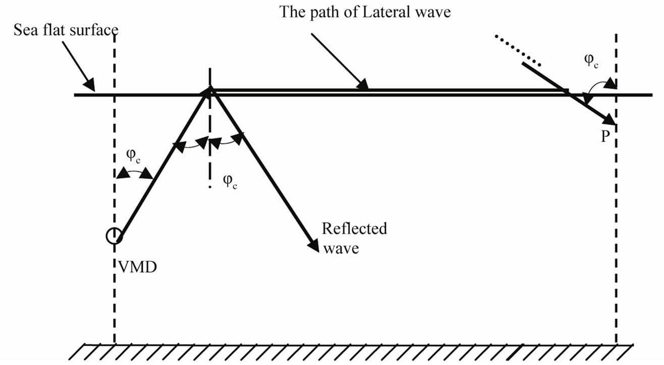
Figure 2. The paths of reflected and lateral waves.
and
 (4)
(4)
where .
.
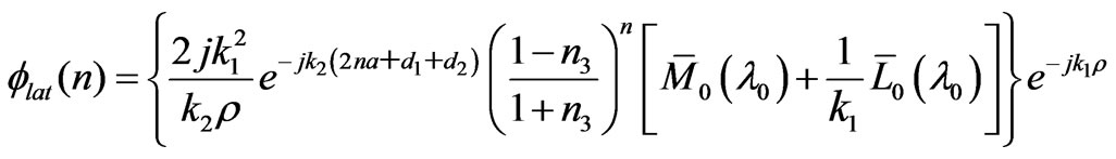
Using the first formula of (4) and rearranging properly
 and
and  to obtain the lateral waves. Then, we have
 (5)
(5)
where
 (6)
(6)
 (7)
(7)
The first factor in (6) is a slowly varying part, while the second term is rapidly varying. The location of the stationary phase point is given by
 (8)
(8)
The solution of (8) is
 (9)
(9)
where,  We can see that the approximation in (9) is valid for
 and
and , then we get
 (10)
(10) where 
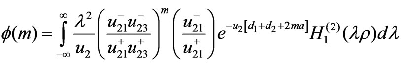
In analogy to this approach we can obtain  as follows
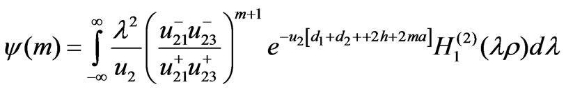
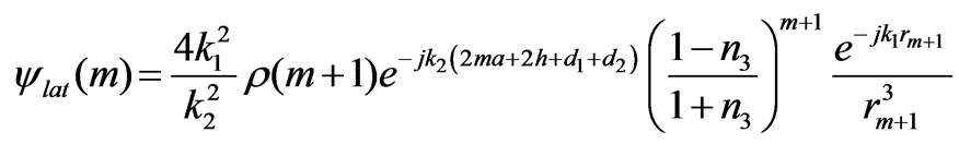 (11)
(11)
From (10) and (11), we get
 (12)
(12)
The exponential in the lateral wave term all indicates that the wave travel vertically a distance  from the dipole to the boundary surface in the sea, then horizontally along the boundary a distance
  in the air, and finally vertically in the sea to the point of observation.
4. Lateral Waves at the Rough Surface of the Sea
In this section we shall calculate the lateral waves for secondary fields in the sea. These will represent the changes which occur in the electromagnetic field of the wave propagation in the sea due to the perturbation applied on the upper surface, where
 (13)
(13)
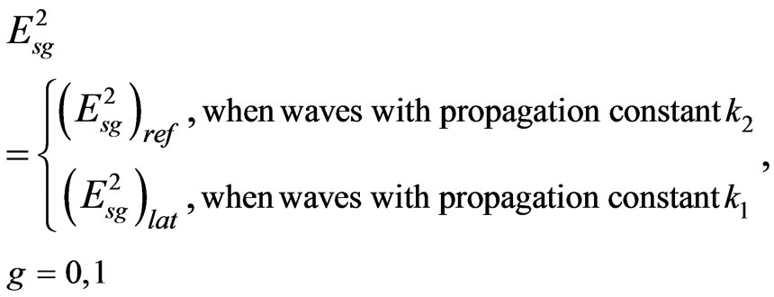
 : The secondary reflected electric field in the sea in any direction,
 : The secondary lateral electric field in the sea in any direction, as in Figure 3.
The reflected field has been calculated in the previous paper [4]. We can calculate
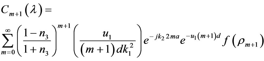
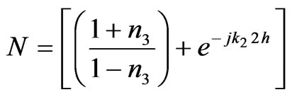
  by using the following approach, in which the denominator can be expanded as an infinite series, i.e.,
 (14)
(14)
Then,
 (15)
(15)
whereIn this research, there is always  for any frequency, therefore, the condition required for (4) is met. Using the first formula of (4) and arranging properly, we get
 , (16)
Figure 3. The paths of reflected and lateral waves.
 (17)
(17)
 (18)
(18)
When , there is an approximate formula for Hankel function as
 .
.
Then, when , the first bracket in
  is slowly varying part while the second bracket is rapidly varying. The location of the stationary phase point in
  is given by:
 (19)
(19)
The solution of (19) is given by
 (20)
(20)
where, . We can see that the approximation in (4) is valid for
 . Apparently the reason of this validity is because the stationary phase point ends up being at
 .
.
Using the approach we presented in the pervious paper [4], we get
 (21)
(21)
Similarly,
 (22)
(22)
Then, from (21) and (22) we get
By using the following approximation,  can be expressed as
 (23)
(23)
In the same way,
 (24)
(24)
Hence,
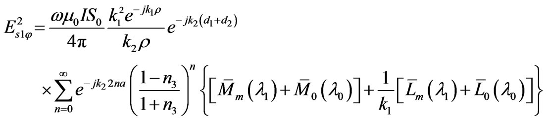 (25)
(25)
where,

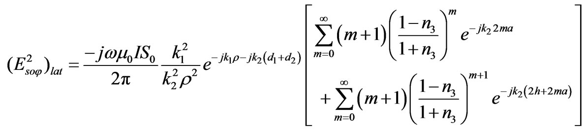
From (25), we have found the lateral waves near the rough surface of the sea. The physical meaning of the first term in (25) indicates a series of waves that propagate upward from the source and make n round trips between the rough sea surface and the bottom, then travel along the surface on the seawater, and finally arrive at the field point in sea, where  is the reflection coefficient at the sea bottom, as in Figure 4.
The second term represents another series of waves that propagate downward from the source first then reflected upward at the sea bottom and travel along the same path. These results also show that  and
and  are proportional with
 , and this means that the electric field in the sea takes the form of the Sommerfeld integral. Also, the result coincides with the result obtained by Long et al. [5], when the disturbed factor
  is neglected.
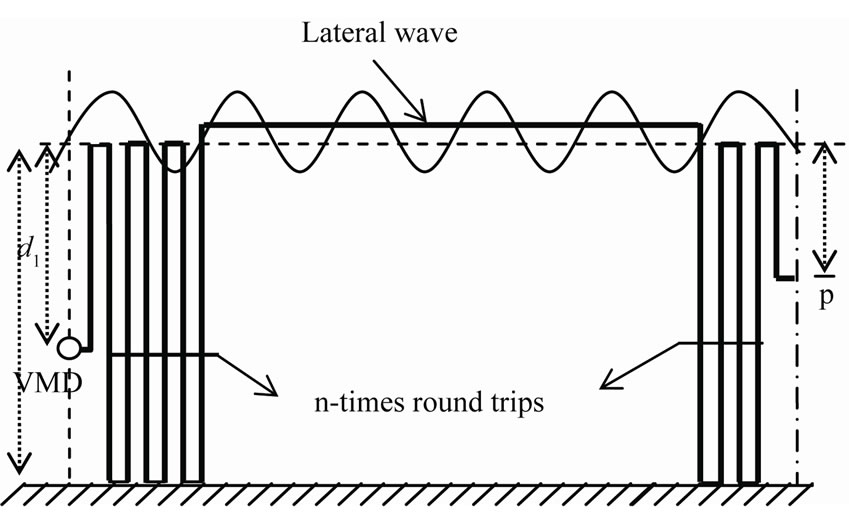
Figure 4. The propagation paths of lateral waves between the source and the bottom to receiver.
5. Numerical Results
The magnitudes of the electric field (the reflected and lateral waves) for the two cases (flat and rough) in sea are computed for different values of the sea thickness and different frequencies.
Case I: Flat surface of the sea: the Figures 5 to 7 show the normalized electric field of the dipole in sea versus the radial distance factor . The depth
  of the field point is taken equal to 5 m. To attain the numerical calculation, we ascertain that
  is a match for
  under the conditions shown in Figures 5 to 7.
We show in these figures that increasing the depth of the sea decreases the value of the electric field. Thus, the previous equations have led to those valid and useful results. These findings also indicate the importance of the derived equations in this research area that could be easily applied in treating related problems.

Figure 5. The reflected waves in sea with uniform surface.
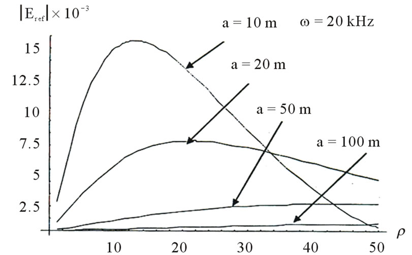
Figure 6. The reflected waves in sea with uniform surface.

Figure 7. The reflected waves in sea with uniform surface.
Plots of the variation of the electric field in the case of the lateral waves are shown in Figures 8 to 10. Also, in these Figures, the numerical calculations ascertain that
 is a match for
 . Also, we show that as the depth of the sea increases, the magnitude of the electric field near the air-sea boundary surface proceeds parallel to the horizontal scale.
In the Figure 5, we consider that the horizontal axis denote the radial distance  and the vertical axis denote the normalized reflected electric field
 . To guarantee that our work proves correctness, we took four different values for the sea depth (a) as shown in Figure 5. The frequency
  was also taken to be 10 KHz. Accordingly, the results show that as we increase the sea depth, the value of the absolute reflected electric field decreases as the radial distance factor
  increases.
Furthermore, we used the same values for the sea depths, but altered the values of the frequency to demonstrate that the absolute reflected electric field increases as we increase the frequency. This is clearly shown in Figures 5-7.
In addition to the reflected wave, we also examined the lateral wave. We used the same sea depth and the same frequencies. Accordingly, we got the previous three Figures 8, 9 and 10. They show that as the sea depth increases and as the frequency decreases, the lateral wave also decreases.
Case II: Rough surface of the sea. The perturbed lateral electric field  for the rough upper surface and reflected electric field
  for the same mode are computed. The part of the sea under investigation takes different thickness (a = 10 m, 25 m, 50 m), the height of the source is taken to be 4 m from the ground (the bottom of the sea). We chose the sea waves represented by the roughness cosine profile with period
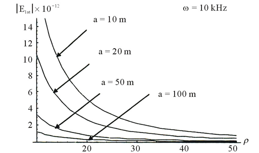
Figure 8. The lateral waves in sea with uniform surface.
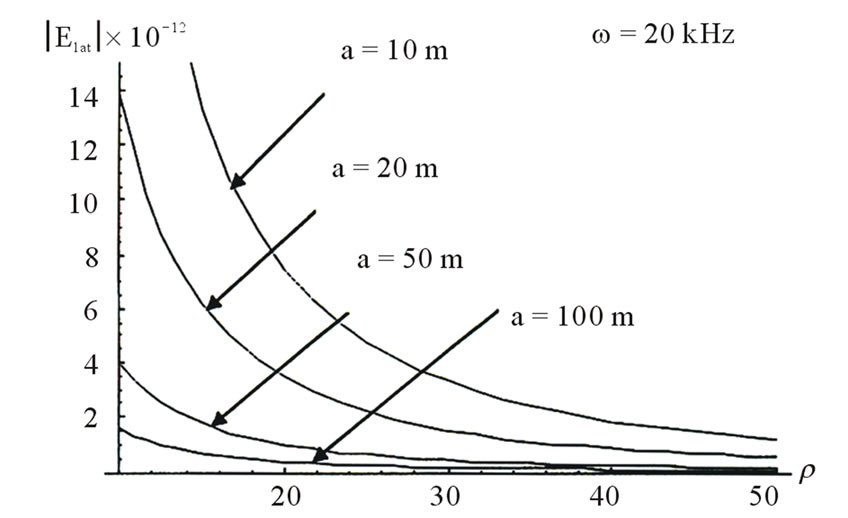
Figure 9. The lateral waves in sea with uniform surface.
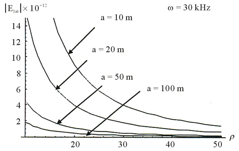
Figure 10. The lateral waves in sea with uniform surface.
10 m and for frequency 10 KHz. Consequently, Figure 11 shows that the reflected waves are decreasing rapidly with the increasing radial distance ρ at different sea depths.
Moreover, in Figure 12 we illustrate that lateral waves act appositely to the reflected waves where they are increasing hastily with the increasing radial distance  at the same different depths.
6. Conclusions
In this paper, we summarized our research work regarding the closed-form expressions for the far fields in the sea. The formulas describe the reflected electric field and the lateral waves near the sea surface for different frequencies 10, 20, 30 KHz. The presented results prove that the lateral waves-in the case of uniform surface are very useful in the navigation with very low frequencies as indicate in Figure 8.
For instance in Figures 8-10, we proved that when we fix the radial distance factor  and the sea depth
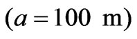 , the lateral waves decreased from 2, 1.5 and 1 as the frequencies decreased from 30, 20 and 10 respectively. Also, from these results we show that the reflected waves can be neglected with respect to the higher values of the lateral waves.
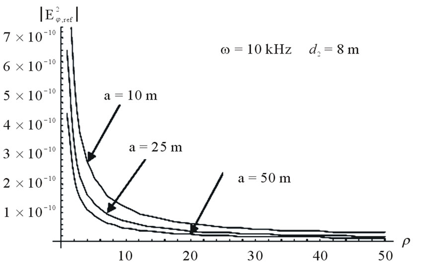
Figure 11. Variation of the absolute value of the reflected electric fields  versus radial distance of the field point for different depths.
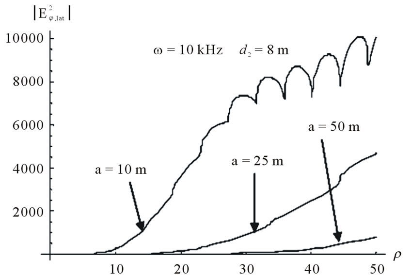
Figure 12. Variation of the absolute value of the lateral electric fields  versus radial distance of the field point for different depths.
REFERENCES
- R. W. P. King, “Lateral Electromagnetic Pulses Generated by a Vertical Dipole on a Plane Boundary between Dielectrics,” Journal of Electromagnetic Waves and Applications, Vol. 2, No. 3-4, 1988, pp. 225-243.
- S. T. Bishay, “Communication of Radio Waves in Sea with a Rough Upper Surface,” AEÜ Archiv Elektronik Übertrag, Vol. 38, No. 3, 1984, pp. 186-188.
- L. El S. Rashid, S. T. Bishay and O. M. Abo-Seida, “Electromagnetic Field Produced by a Vertical Magnetic Dipole above a Rough Surface,” Proceeding of the International Conference on Electromagnetics in Advanced Applications, 12-15 September 1995, pp. 231-240.
- O. M. Abo-Seida, S. T. Bishay and K. M. El-Morabie, “Far-Field Radiated from Vertical Magnetic Dipole in Sea with a Rough Upper Surface,” IEEE Transactions on Geoscience and Remote Sensing, Vol. 44, No. 8, 2006, pp. 2135-2142. doi:10.1109/TGRS.2006.872135
- Y. Long, H. Jiang and B. Rembold, “Far-region Electromagnetic Radiation with a Vertical Magnetic Dipole in Sea,” IEEE Transactions on Antennas Propagation, Vol. 49, No. 6, 2001, pp. 992-996. doi:10.1109/8.931158
- W. C. Chew, “A Quick Way to Approximate a Sommerfeld-Weyl-Type Integral,” IEEE Transactions on Antennas Propagation, Vol. 36, No. 11, 1988, pp. 1654-1657. doi:10.1109/8.9724
- P. R. Bannister, “The Image Theory of Electromagnetic Field of a Horizontal Electric Dipole in the Presence of a Conducting Half-Space,” Radio Science, Vol. 17, No. 5, 1982, pp. 1095-1102. doi:10.1029/RS017i005p01095
Appendix A
where  is the location of the stationary phase point which is given by
 .
.
The prime  and
and  denote differentiation of
  with respect to
  and
and  and
and .
.


 .
.