Journal of Electromagnetic Analysis and Applications
Vol. 2 No. 10 (2010) , Article ID: 2984 , 6 pages DOI:10.4236/jemaa.2010.210079
An Analysis of Interference as a Source for Diffraction
![]()
Consultant, Lasers and Electrooptics Montreal, Canada.
Email: chamonix@total.net
Received September 1st, 2010; revised September 29th, 2010; accepted October 6th, 2010.
Keywords: Electromagnetic Wave Analysis, Diffraction Phenomena, Interference
ABSTRACT
An analysis is made of interference of two plane waves which in turn give rise to subsequent diffraction phenomena. This is done using two different approaches. One of them is straight forward but is difficult to interpret. The second is less conventional but more intuitive thus giving more insight into the process. The geometry is kept very simple to focus on the process itself. Both approaches give rise to the same results thus offering a choice in tackling such problems.
1. Introduction
Interference and diffraction theory have been developed as a result of the realization of the wavelike nature of light. This has led to the thousands of successful applications, ranging from the many forms of interferometers to the development of optical components such as Fresnel lenses and other Fourier transform components, making possible the wide field of present day Photonics.
The basics of interference and diffraction theory can easily be obtained from textbooks [1,2]. To get a better insight into these phenomena, however, would require a closer examination, such as, by looking at them from different perspectives.
The purpose of this paper is to provide such an insight by looking at a simple situation comprising an interference situation, which in turns gives rise to a diffraction phenomenon. The problem is then solved using two different approaches. Although the first is more straightforward, the results are difficult to interpret. The second, is less conventional but more intuitive. The geometry is kept very simple to focus on the process itself. It consists of a wall on which two plane waves intersect to form interference fringes, a slit in the wall through which the interference wave passes and a screen at a distance behind the wall which exhibits the resulting diffracted wave that was produced by the slit. Waveforms are calculated at the wall and at the screen for each of the two approaches and compared. The second approach is then used to offer an insight for the solution obtained by the first approach. The power transfer is calculated for each approach to ascertain that the process obeys conservation of energy.
As an example, we shall discuss how two beams intersecting and thus interfering at a point behave as they move away from it.
As both approaches give rise to the same results, a side benefit of this analysis is that it provides a choice in tackling such problems depending on the type of initial information that is supplied.
2. Configuration Selection
Referring to Figure 1, we assume two infinite plane waves with amplitude E1 and E2 , polarized in the Y direction (which is perpendicular to the paper), with their normals in the XZ plane approaching an infinitely large wall in the XY plane at Z = 0. Their normals make an angle i and –i with the Z-axis respectively. It is further assumed that the wall has an infinitely long slit in the Y direction of width “a” along the X-axis centered at Xw = 0. On the right of the slit, a large screen, parallel to the wall, is placed at a distance “d” from it.
For discussion purpose, we have chosen the distance d so that the geometrical overlap of the two beans entering the slit and reaching the screen has a width a/2 along the Xs ordinate.
It is to be expected that there will be interference effect at the wall due to the superposition of the two waves which will result in fringes on the wall. In particular, this interference field will penetrate the slit and end up on the
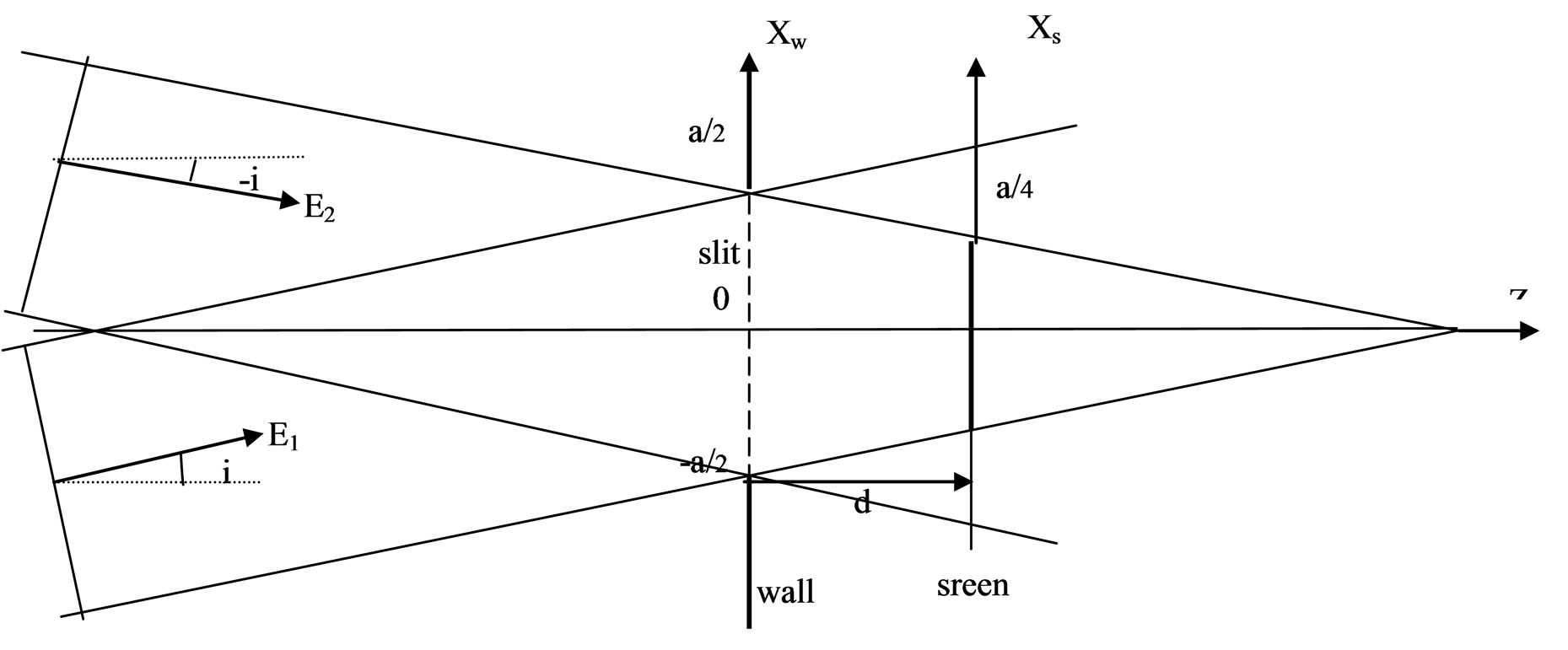
Figure 1. Two plane waves E1 and E2 intersect on a wall at Z = 0, enter through a slit of width a and are projected on a screen at Z = d.
screen. We shall calculate, using two different approaches, the resulting field at the screen and compare the results.
2.1. Approach 1
Starting with what we consider the most straightforward approach, we shall calculate first the interference field at the slit. Since, on entering the slit, it is being sliced by its edges, which we assume to be very thin, we expect diffraction to take place. We shall then use diffraction theory to calculate the resulting field at the screen originating from this interference field.
2.2. Approach 2
We follow each plane wave separately, obtain their field strength at the slit, noting that each wave has been sliced by the slit, and calculate the resulting field at the screen as caused by diffraction. We end up with two separate diffracted fields at the screen originating from the two original plane waves. We then calculate the interference field resulting from their superposition. We compare the results with those of Approach 1 to ensure that they are the same.
3. Relevant Theory
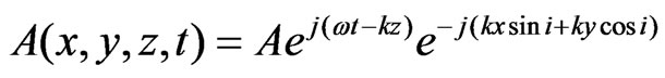
Following Approach 1, let the two plane waves approaching the wall have a functional representation given by [3],
 (1)
(1)
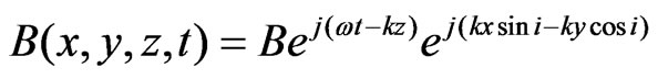 (2)
(2)
where A and B are amplitude constants proportional to the fields E1 and E2 respectively. They will be evaluated later. Since we want to calculate the interference field at the wall (including the slit), we know that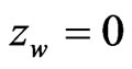 . Also, since the field amplitude is invariable along the Y direction, we let y = 0. Adding Equations (1) and (2) we get the amplitude of the interference field at the wall to be,
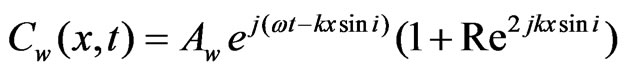 (3)
(3)
where R = Bw/Aw.
To relate Aw and Bw to the actual field, we shall resort to the conservation of energy principle. To do this we note that the intensity at the wall of this interference field is given by the time average of the square of Equation (3) which is well know to require a factor of ½ to the result. The intensity is therefore given by,
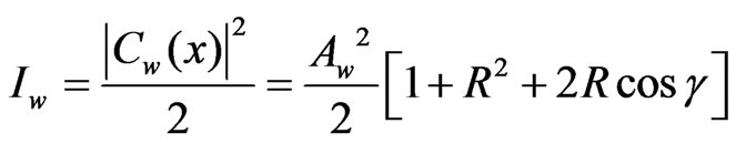 (4)
(4)
where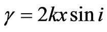 . The total power entering the slit per unit length in the Y direction is therefore,
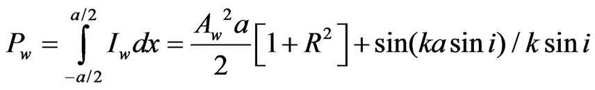 (5)
(5)
To simplify our interpretation, we want to examine only whole fringes. This will occur when the last term, which is associated with partial fringes, is made equal to zero. This occurs when  where
where  or
or
 (6)
(6)
With n representing the number of whole fringes. The total power per unit length at the slit is,
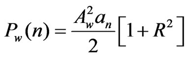 (7)
(7)
We are now prepared to relate Aw and Bw to the fields. Looking back at field E1 in Figure 1, its related intensity is defined as the energy transmitted per sec per unit area normal to the direction of propagation. It is proportional to E12/2. But the wall is not normal to the direction of the plane wave. The intensity along the wall is spread out over a larger area by a factor of 1/cos i. The power associated with plane wave E1 per unit of Y is therefore proportional to . Similarly, the power associated with E2 is
 . The total power entering the slit from both waves per units of Y is thus
 (8)
(8)
Comparing Equations (7) and (8) which should be equal for conservation of energy, we must have  and
and (9)
(9)
Before we can calculate the field at the screen using diffraction theory, we need the amplitude and phase of the field at the slit. We obtain it from Equation (3) by rewriting it as,
 (10)
(10)
where  and
and and
and  is the argument of D(x), or the angle the phasor D(x) makes with the X‑axis. The term
  has been omitted since it is common to all the expressions and is of no importance to calculate the amplitude at the screen. Since the field at the slit is being clipped by the edge of the slit, we shall use the Fresnel-Kirckhoff formulation of diffraction theory [1]. We assume that the two plane waves have their field polarized in the Y direction so that Ex = Ez =0. Further, the slit at the wall is assumed to be infinite in length in the Y direction. This simplifies somewhat the mathematics since the field should be invariable in that direction. Consequently, we shall use the simplified one-dimensional expression [4],
 , (11)
Where Cs is the field disturbance resulting from that at the slit, d is the distance between the wall and the screen, 
 ,
,  is the angle between the wavefront at xw and the wall normal. It can be obtained from the relation
 .
.
Equation (11) is a good approximation provided that d > a , a > λ , and the angle i is small.
Other approximations would provide similar results [5- 7].
4. Numerical Calculations
For definiteness we let i = 10o, E1 =1, a = 72 and d = 102 both in wavelength units. This will ensure the geometry given in Figure 1.
4.1. Approach 1
In this approach, we calculate first the amplitude of the interference field present at the slit. It is the resultant of the superposition the two plane waves. It can be obtained from Equation (3) by taking its absolute value,
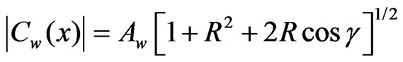 (12)
(12)
This is the interference field, which is responsible for the visible fringes, given by Equation (4).
Plotting the interference field at the slit as a function of xw, which is the normalized distance along the slit, we obtain the waveform shown as curve (a) in Figure 2. we note first that there are 25 peaks present at the slit as should be expected, the slit extends in the range -36 < xw < 36. for a total width of 72 wavelengths. The amplitude varies from 0 to 2 Aw.
We can now use the interference field Equation (3) at the slit to calculate how it is transformed when it reaches the screen. For this we use the appropriate diffraction expression Equation (11) since the field is sliced by the edges of the slit. It turns out that for R = 1, φw = 0 for all values of xw. Using computer numerical calculations, we obtain the field at the screen which is plotted on the same graph in Figure 2 as curve (b) for comparison purpose.
We observe that around the central portion of the screen, the waveform pattern is very similar in shape and amplitude to that at the slit. As we move away from this region, the field amplitude falls down to a level somewhat half-way down until around Xs = 50 when it decreases very quickly in amplitude towards zero. Also, the distance between peaks increased compared to that at the slit. To explain quantitatively the behaviour of the waveform from this approach is not simple. On the other hand, when Approach 2 is used, a much more intuitive derivation will permit a better understanding of the process.
4.2. Approach 2
In this approach, we follow each plane wave separately as they reach the slit. Since they are sliced by the slit, we can use diffraction theory to calculate their resulting fields at the screen. We then add these fields (which are phasors) to obtain the combined field. The results are then compared with that of Approach 1.
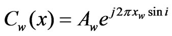
Starting with plane wave E1, we notice that when it reaches the wall, its amplitude is obviously a constant, although its phase varies with Xw. Cw simplifies now to,
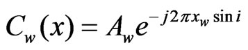 . (13)
This is shown in Figure 3-curve (a).
Since in this case φ = i = 10o, using Equation (11) we obtain the diffracted field amplitude at the screen shown as curve (b). As should be expected, this is a typical wave-
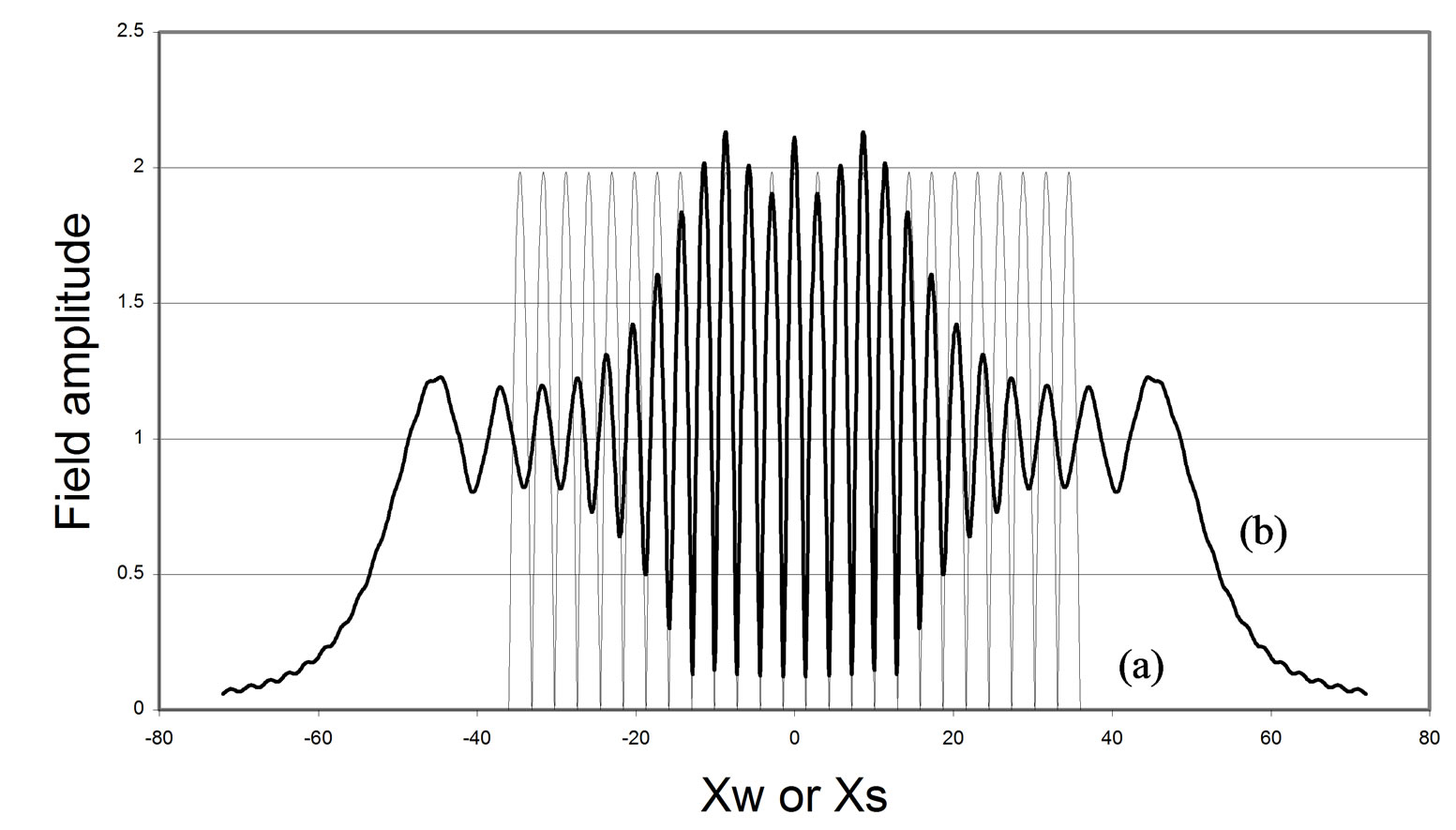
Figure 2. Field amplitude in arbritrary units of two plane waves E1 and E2 meeting at a slit as a function of position in wavelength units. (a) interference field at wall slit along Xw; (b) diffration field at screen along Xs.
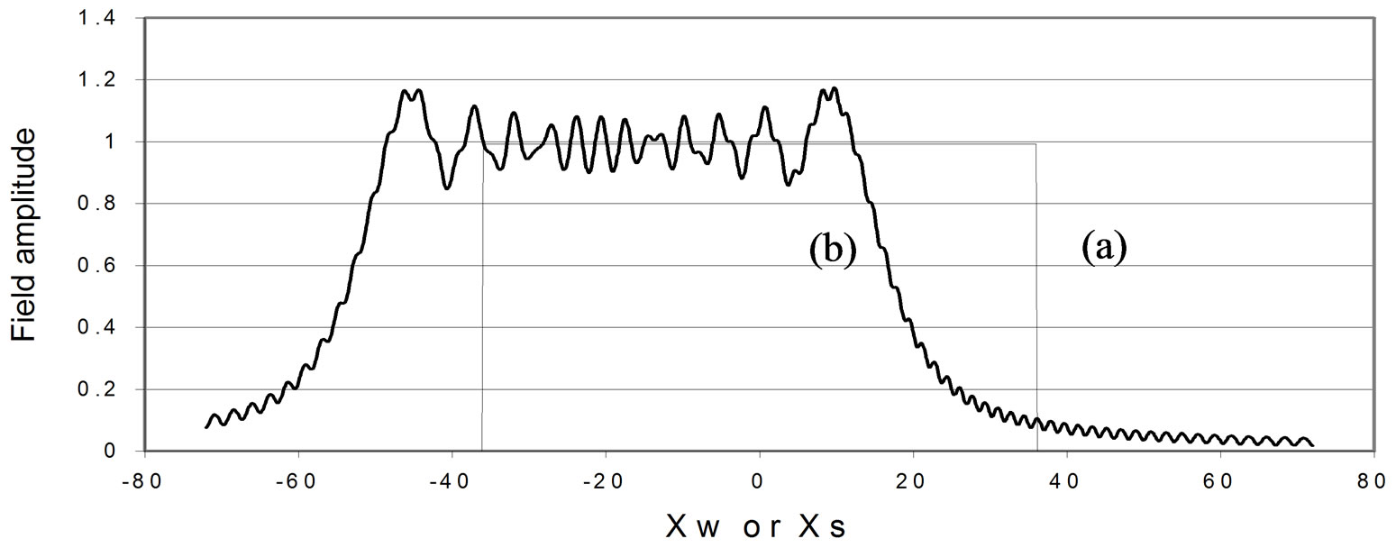
Figure 3. Field amplitude in arbitrary units of plane wave E1 meeting at a slit as a function of position in wavelength units.
(a) field at wall slit along Xw from plane wave E1; (b) resulting diffration field at screen along Xs.
form of Fresnel diffraction by a slit. It is, however, displaced by 10o to the left of center. Obviously, a similar waveform is produced by plane wave 2, except that it is displaced by the same amount to the right. Its function at the wall is,
 . (14)
If the two diffracted fields are added, the end result is shown in Figure (4) as curve (d). A comparison with Figure 2 curve (b) shows that they are identical.
To get an intuitive understanding of that curve, we now plot on the same graph the waveforms of plane wave E1 shown in Figure 3 as curves (a) and (b). For reference purpose, curve (c) is added and is the interference field the two plane waves shown in Figure 2 curve (a). Finally, we recall that in Section II we have selected the distance d so that the geometric overlap of the two waves at the screen covers only half the width of the slit. This is shown as region (e). We thus observe that, for the main diffraction curve (d):
1) At the edge of the waveform, on the left of the Figure, away from region (e), where there is no overlap, the shape follows almost exactly the waveform of a single plane wave - curve (b).
2) In region (e), the center portion where there is overlap, the shape is essentially that due to the sum of the two incoming waves.
3) In between those two regions, the wave progressively changes in shape and amplitude to blend from the overlap to the single wave region.
4) We should be gratified that our results show that in the region, away from (e), where there is no overlap, the waveform reverts to that of single plane waves. This is because we know from intuition, that if two beams cross

Figure 4. Field amplitude of plane wave(s) as a function of position for situations: (a) field at wall slit from plane wave E1 along Xw; (b) diffraction field as a result of (a) at sceen along Xs; (c) interference field at wall slit along Xw resulting from both E1 and E2; (d) diffraction field at screen along Xs resulting from adding curve (b) from E1 and its counter part from E2; (e) geometric overlap of E1 and E2 at the screen.
one another, they will eventually carry on as if the interference region was not there. It should be emphasized, of course, that this is only true if the interference takes place in a vacuum where no other interaction takes place.
Approach II thus allows us to see why the shape of the diffracted wave derived in Approach I can be evolved from the diffracted waves produced by the two individual plane waves.
5) Power Transfer Considerations We have shown, so far, that Approaches 1 and 2, although quite different, give out the same results as far as final waveforms at the screen are concerned. As a final check, we would like to ascertain that the power entering the slit is equal to the power reaching the screen for both Approaches for conservation of energy.
The initial power from the two incoming waves entering the slit per unit length in the Y direction is given by Equation (7). The intensity at the screen is given by
 (15)
(15)
where Cs is the total field obtained from Equation (11) for each of the approaches, while φs is the angle between the resulting field at xs and the Z-direction. The total power per unit length in the Y direction in each case is then obtained by integrating,
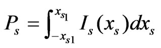 (16)
(16)
Where xs1 is taken far enough from xs = 0 that the field is negligible.
When the calculations are performed, it is found that the difference in power between the incoming power at the slit and that at the screen for both Approaches is of the order of 1%. This is well within the approximations expected from Equation (11).
6. Conclusion
We have considered interference theory resulting from two plane waves meeting at a slit, and on entering it, being subjected to the diffraction phenomenon. This was done using a simple geometry to focus on the process itself. Two approaches were selected, one more intuitive than the other. We have seen that they provide essentially the same results. Approach 2 which is more intuitive helps to understand the former which is more conventional but more difficult to visualize. It also demonstrate that interference effect in a vacuum, although manifesting itself mainly in a region of beam overlap, does not carry a permanent effect on the beams which revert back to their original behavior once they move far enough away from the overlapped region.
As a corollary to the calculations for both approaches, we have demonstrated, by an example, that the interference field which is made up of the superposition of two or more fields can be used as the starting source to calculate further diffraction effects caused by obstacles. On the other hand, if the components of the interference field reaching the obstacle are known, each of the components can be used to calculate its diffraction effect. The sum of the diffracted fields will then give rise to the same results as in the first case. Consequently, this suggests that a choice can be made in solving such problems based on the type of initial information that is supplied.
As a final remark, although we have considered in this paper only cases where R = 1 and 0, it can be shown that similar conclusions can be obtained for other values of R.
REFERENCES
- M. Born and E. Wolf, “Principle of Optics,” Pergamon Press, New York, 1970.
- S. Silver, “Microwave Antenna Theory and Design,” Dover, New York, 1965.
- C. Slater and N. Frank, “Electromagnetism,” McGraw Hill, New York, 1947.
- A. Fox and T. Li, “Resonant Modes in a Maser Interferometer,” Bell System Technical Journal, Vol. 40, 1961, pp. 453-488.
- K. Mielenz, “Algorithms for Fresnel Diffraction at Rectangular and Circular Apertures,” Journal of Research of the National Institute Standards and Technology, Vol. 103, No. 5, 1998, pp. 497-509.
- K. Abedin, “Computer Simulation of Fresnel Diffraction from Rectangular Apertures and Obstacles Using the Fresnel Integrals Approach,” Optics and Laser Technology, Vol. 39, No. 2, 2007, pp. 237-246.
- A. Waksberg, “FIR Laser Efficiency Enhancement by Double Resonance Tuning,” International Journal of Infrared and Millimetre Waves, Vol. 26, No. 3, 2003, pp. 363-373.