Journal of Intelligent Learning Systems and Applications
Vol.6 No.1(2014), Article ID:42869,8 pages
DOI:10.4236/jilsa.2014.61005
Support Vector Machine and Random Forest Modeling for Intrusion Detection System (IDS)
1Department of Computer Science and Engineering, Rajshahi University
of Engineering and Technology (RUET), Rajshahi, Bangladesh;
2Department
of Statistics, University of Rajshahi, Rajshahi, Bangladesh;
3Department
of Computer Science and Engineering, University of Rajshahi, Rajshahi, Bangladesh.
Email: mehedi_ru@yahoo.com, mnasser.ru@gmail.com, biprodip.cse@gmail.com, shamim_cst@yahoo.com
Copyright © 2014 Md. Al Mehedi Hasan et al. This is an open access article distributed under the Creative Commons Attribution License, which permits unrestricted use, distribution, and reproduction in any medium, provided the original work is properly cited. In accordance of the Creative Commons Attribution License all Copyrights © 2014 are reserved for SCIRP and the owner of the intellectual property Md. Al Mehedi Hasan et al. All Copyright © 2014 are guarded by law and by SCIRP as a guardian.
Received June 29th, 2013; revised July 29th, 2013; accepted August 7th, 2013
KEYWORDS
Intrusion Detection; KDD’99; SVM; Kernel; Random Forest
ABSTRACT
The success of any Intrusion Detection System (IDS) is a complicated problem due to its nonlinearity and the quantitative or qualitative network traffic data stream with many features. To get rid of this problem, several types of intrusion detection methods have been proposed and shown different levels of accuracy. This is why the choice of the effective and robust method for IDS is very important topic in information security. In this work, we have built two models for the classification purpose. One is based on Support Vector Machines (SVM) and the other is Random Forests (RF). Experimental results show that either classifier is effective. SVM is slightly more accurate, but more expensive in terms of time. RF produces similar accuracy in a much faster manner if given modeling parameters. These classifiers can contribute to an IDS system as one source of analysis and increase its accuracy. In this paper, KDD’99 Dataset is used and find out which one is the best intrusion detector for this dataset. Statistical analysis on KDD’99 dataset found important issues which highly affect the performance of evaluated systems and results in a very poor evaluation of anomaly detection approaches. The most important deficiency in the KDD’99 dataset is the huge number of redundant records. To solve these issues, we have developed a new dataset, KDD99Train+ and KDD99Test+, which does not include any redundant records in the train set as well as in the test set, so the classifiers will not be biased towards more frequent records. The numbers of records in the train and test sets are now reasonable, which make it affordable to run the experiments on the complete set without the need to randomly select a small portion. The findings of this paper will be very useful to use SVM and RF in a more meaningful way in order to maximize the performance rate and minimize the false negative rate.
1. Introduction
Along with the benefits, the Internet also created numerous ways to compromise the stability and security of the systems connecting to it. Although static defense mechanisms such as firewalls and software updates can provide a reasonable level of security, more dynamic mechanisms such as intrusion detection systems (IDSs) should also be utilized [1]. Intrusion detection is the process of monitoring events occurring in a computer system or network and analyzing them for signs of intrusions. IDSs are simply classified as host-based or network-based. The former operates on information collected from an individual computer system and the latter collects raw network packets and analyzes for signs of intrusions. There are two different detection techniques employed in IDS to search for attack patterns: Misuse and Anomaly. Misuse detection systems find known attack signatures in the monitored resources. Anomaly detection systems find attacks by detecting changes in the pattern of utilization or behavior of the system [2].
As network attacks have increased in number and severity over the past few years, Intrusion Detection Systems (IDSs) have become a necessary addition to the security infrastructure of most organizations [3]. Deploying highly effective IDS systems is extremely challenging and has emerged as a significant field of research, because it is not theoretically possible to set up a system with no vulnerabilities [4]. Several machine learning (ML) algorithms, for instance Neural Network [5], Genetic Algorithm [6], Fuzzy Logic [4,7-9], clustering algorithm [10] and more have been extensively employed to detect intrusion activities from large quantity of complex and dynamic datasets.
In recent time, SVM and RF have been extensively applied to providing potential solutions for the IDS problem. This paper is focused on the analysis of the performance of two commonly used data mining techniques: SVMs [11] and Random Forests (RF) [12]. KDD’99 dataset has been used to train and test the model. The effectiveness and the efficiency of classification modeling are then empirically analyzed.
The remainder of the paper is organized as follows. Section 2 provides the description of the KDD’99 dataset. We outline mathematical overview of SVM and RF in Section 3. Experimental setup ispresentedin Section 4 and Preprocessing, Evaluation Metrics and SVM model selection are drawn in Sections 5, 6 and 7 respectively. Finally, Section 8 reports the experimental result followed by conclusion in Section 9.
2. KDDCUP’99 Dataset
Under the sponsorship of Defense Advanced Research Projects Agency (DARPA) and Air Force Research Laboratory (AFRL), MIT Lincoln Laboratory has collected and distributed the datasets for the evaluation of researches in computer network intrusion detection systems [13]. The KDD’99 dataset is a subset of the DARPA benchmark dataset prepared by Sal Stofo and Wenke Lee [14]. The KDD dataset was acquired from raw tcpdump data for a length of nine weeks. It is made up of a large number of network traffic activities that include both normal and malicious connections. A connection in the KDD’99 dataset is represented by 41 features, each of which is in one of the continuous, discrete and symbolic form, with significantly varying ranges. The KDD’99 dataset includes three independent sets: “whole KDD”, “10% KDD”, and “corrected KDD”. Most of researchers have used the “10% KDD” and the “corrected KDD” as training and testing set, respectively [15]. The training set contains a total of 22 training attack types. The “corrected KDD” testing set includes an additional 17 types of attacks and excludes 2 types (spy, warezclient) of attacks from training set, therefore, there are 37 attack types those are included in the testing set, as shown in- Tables 1 and 2. The simulated attacks fall in one of the four categories [1,15]: 1) Denial of Service Attack (DoS); 2) User to Root Attack (U2R); 3) Remote to Local Attack (R2L); 4) Probing Attack.
Inherent Problems of the KDD’99 and Our Proposed Solution
Statistical analysis on KDD’99 dataset found important issues which highly affects the performance of evaluated systems and results in a very poor evaluation of anomaly detection approaches [16]. The most important deficiency in the KDD dataset is the huge number of redundant records. Analyzing KDD train and test sets, Mohbod Tavallaeefound that about 78% and 75% of the records are duplicated in the train and test set, respectively [17]. This large amount of redundant records in the train set
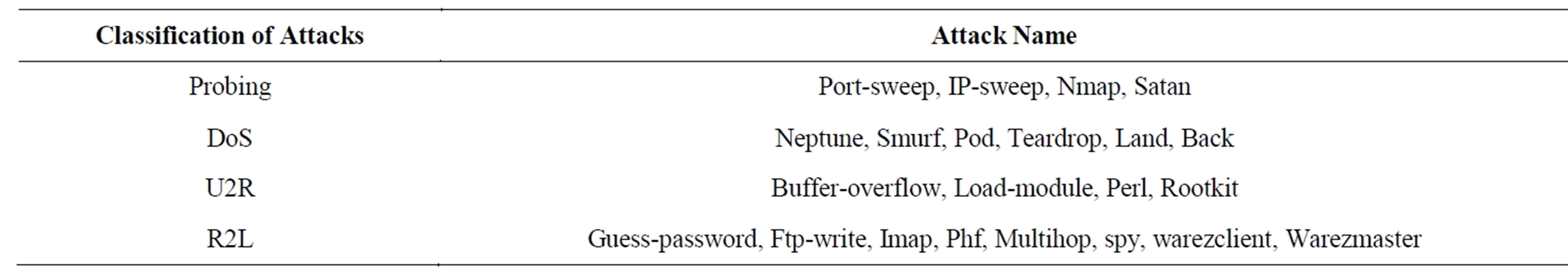
Table 1. Attacks in KDD’99 Training dataset.
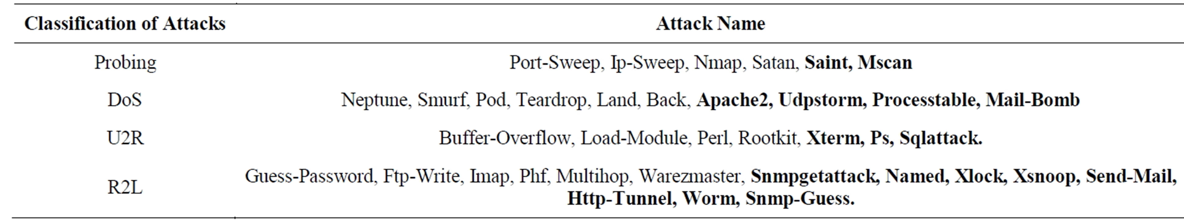
Table 2. Attacks in KDD’99 Testing dataset.
will cause learning algorithms to be biased towards the more frequent records, and thus prevent it from learning unfrequent records which are usually more harmful to networks such as U2R attacks. The existence of these repeated records in the test set, on the other hand, will cause the evaluation results to be biased by the methods which have better detection rates on the frequent records.
To solve these issues, we have derived a new dataset by eliminating redundant record from KDD’99 train and test dataset (10% KDD and corrected KDD), so the classifiers will not be biased towards more frequent records. This derived dataset consists of KDD99Train+ and KDD99Test+ dataset for training and testing purposes, respectively. The numbers of records in the train and test sets are now reasonable, which makes it affordable to run the experiments on the complete set without the need to randomly select a small portion.
3. Classification
Consider the problem of separating the set of training vectors belong to two separate
classes,
 where
where
 and
and
 is the corresponding class label, 1 ≤ i ≤ n. The main task is to find a classifier
with a decision function f(x, θ) such that y = f(x, θ), where y is the class label
for x, θ is a vector of unknown parameters in the function.
is the corresponding class label, 1 ≤ i ≤ n. The main task is to find a classifier
with a decision function f(x, θ) such that y = f(x, θ), where y is the class label
for x, θ is a vector of unknown parameters in the function.
3.1. SVM Classification
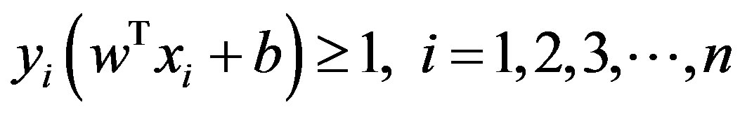
The theory of SVM is from statistics and the basic principle of SVM is finding the optimal linear hyperplanein the feature space that maximally separates the two target classes [17,18]. Geometrically, the SVM modeling algorithm finds an optimal hyperplane with the maximal margin to separate two classes, which requires to solve the following constraint problem can be defined as follows

Subject to:
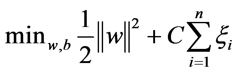
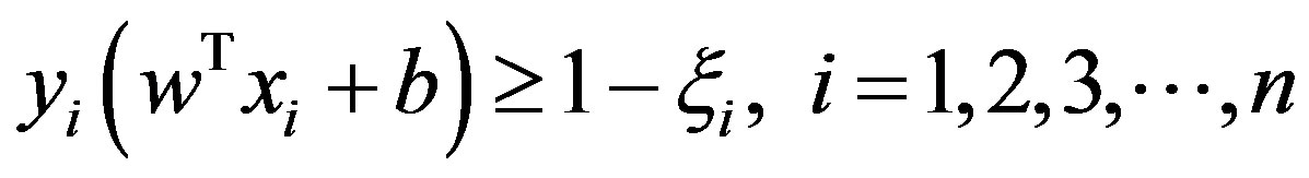
To allow errors, the optimization problem now becomes:
Subject to:
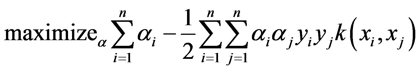
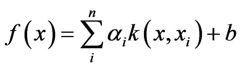
Using the method of Lagrange multipliers, we can obtain the dual formulation which is expressed in terms of variables αi [17,18]:
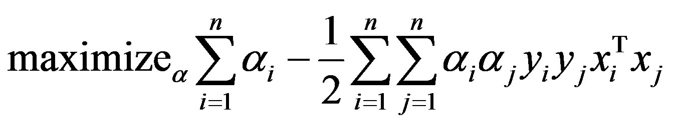
Subject to: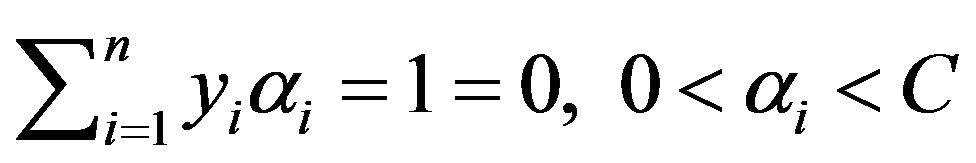
for all

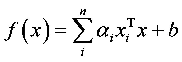
Finally, the linear classifier based on a linear discriminant function takes the following form
In many applications a non-linear classifier provides better accuracy. The naive
way of making a non-linear classifier out of a linear classifier is to map our data
from the input space X to a feature space F using a non-linear function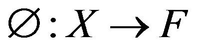 . In the space F,
the optimization takes the following form using kernel function [19]:
. In the space F,
the optimization takes the following form using kernel function [19]:
Subject to: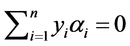 ,
,
for all
Finally, in terms of the kernel function the discriminant function takes the following form:
In this work, Gaussian kernel has been used to build SVM classifier.
Gaussian kernel:
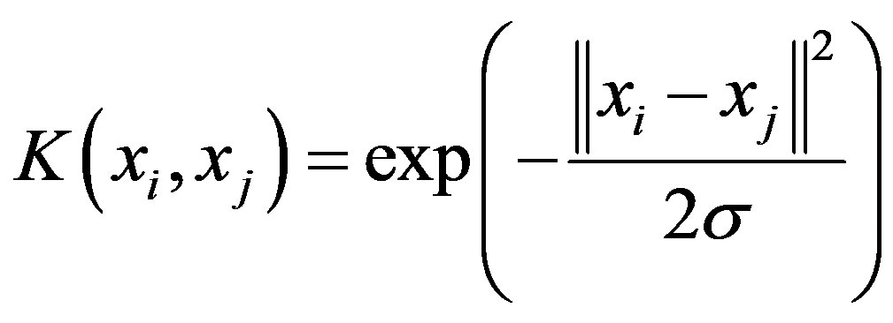 ,
,
 is the width of the function.
A kernel function and its parameter have to be chosen to build a SVM classifier
[20]. Training an SVM finds the large margin hyperplane, i.e. sets the parameters . The SVM has another set of parameters called
hyperparameters: The soft margin constant, C, and any parameters the kernel function
may depend on (width of a Gaussian kernel) [21].
. The SVM has another set of parameters called
hyperparameters: The soft margin constant, C, and any parameters the kernel function
may depend on (width of a Gaussian kernel) [21].
SVMs are formulated for two class problems. But because SVMs employ direct decision functions, an extension to multiclass problems is not straightforward [22]. There are several types of SVMs that handle multiclass problems. We have used here only One-vs-All multiclass SVMs for our research work.
3.2. Random Forest
The random forests [12] is an ensemble of unpruned classification or regression trees. Random forest generates many classification trees. Each tree is constructed by a different bootstrap sample from the original data using a tree classification algorithm. After the forest is formed, a new object that needs to be classified is put down each of the tree in the forest for classification. Each tree gives a vote that indicates the tree’s decision about the class of the object. The forest chooses the class with the most votes for the object.
The random forests algorithm (for both classification and regression) is as follows [23-25]:
1) From the Training of n samples draw ntree bootstrap samples.
2) For each of the bootstrap samples, grow classification or regression tree with the following modification: at each node, rather than choosing the best split among all predictors, randomly sample mtry of the predictors and choose the best split from among those variables. The tree is grown to the maximum size and not pruned back. Bagging can be thought of as the special case of random forests obtained when mtry = p, the number of predictors.
3) Predict new data by aggregating the predictions of the ntree trees (i.e., majority votes for classification, average for regression).
There are two ways to evaluate the error rate. One is to split the dataset into training part and test part. We can employ the training part to build the forest, and then use the test part to calculate the error rate. Another way is to use the Out of Bag (OOB) error estimate. Because random forests algorithm calculates the OOB error during the training phase, we do not need to split the training data. In our work, we have used both ways to evaluate the error rate.
There are three tuning parameters of Random Forest: number of trees (ntree), number of descriptors randomly sampled as candidates for splitting at each node (mtry) and minimum node size [24]. When the forest is growing, randomfeatures are selected at random out of the all features in the training data. The number of features employed in splitting each node for each tree is the primary tuning parameter (mtry). To improve the performance of random forests, this parameter should be optimized. The number of trees (ntree) should only be chosen to be sufficiently large so that the OOB error has stabilized. In many cases, 500 trees are sufficient (more are needed if descriptor importance or molecular proximity is desired). There is no penalty for having “too many” trees, other than waste in computational resources, in contrast to other algorithms which require a stopping rule. Another parameter, minimum node size, determines the minimum size of nodes below which no split will be attempted. This parameter has some effect on the size of the trees grown. In Random Forest, for classification, the default is 1, ensuring that trees are grown to their maximum size and for regression, the default is 5 [24].
4. Dataset and Experimental Setup
Investigating the existing papers on the anomaly detection which have used the KDD dataset, we found that a subset of KDD’99 dataset has been used for training and testing instead of using the whole KDD’99 dataset [16, 26-28]. Existing papers on the anomaly detection mainly used two common approaches to apply KDD’99 [26]. In the first, KDD’99 training portion is employed for sampling both the train and test sets. However, in the second approach, the training samples are randomly collected from the KDD’99 train set, while the samples for testing are arbitrarily selected from the KDD’99 test set. The basic characteristics of the original KDD’99 and our duplicate less (KDD99Train+ and KDD99Test+)intrusion detection datasets in terms of number of samples is given in Table 3. Although the distribution of the number of samples of attack is different on different research papers, we have used the Tables 1 and 2 to find out the distribution of attack [1,3,15]. In our experiment, whole train (KDD99Train+) dataset has been used to train our classifier and the test (KDD99Test+) set has been used to test the classifier. All experiments were performed using Intel core i5 2.27 GHz processor with 4GB RAM, running Windows 7.
To select the best model in model selection phase, we have drawn 10% samples from the training set (KDDTrain+) to tune the parameters of all kernel and another 10% samples from the training set (KDDTrain+) to validate those parameters, as shown in Table 3.
5. Pre-Processing
SVM classification system is not able to process KDD99Train+ and KDD99Test+ dataset in its current format. SVM requires that each data instance is represented as a vector of real numbers. Hence preprocessing was required before SVM classification system could be built. Preprocessing contains the following processes: The features in columns 2, 3, and 4 in the KDD’99 dataset are the protocol type, the service type, and the flag, respectively. The value of the protocol type may be tcp, udp, or icmp; the service type could be one of the 66 different network services such as http and smtp; and the flag has 11 possible values such as SF or S2. Hence, the categorical features in the KDD dataset must be converted into a numeric representation. This is done by the usual binary encoding—each categorical variable having possible m values is replaced with m − 1 dummy variables. Here a dummy variable have value one for a specific category and having zero for all category. After converting category to numeric, we got 115 variables for each samples of the dataset. Some researchers used only integer code
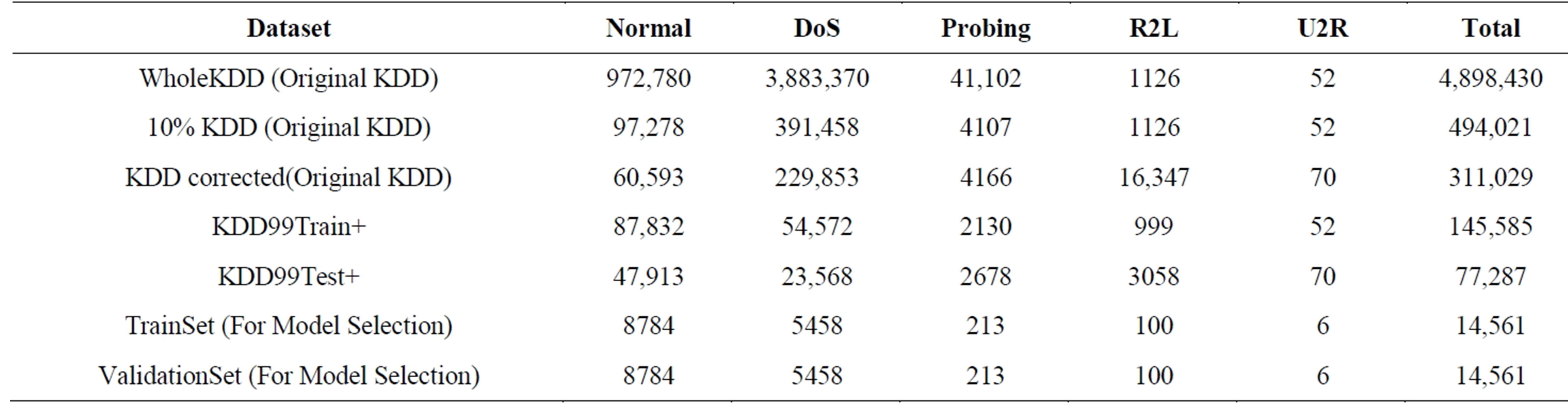
Table 3. Number of samples of each attack in dataset.
to convert category features to numeric representation instead of using dummy variables which is not statistically meaningful way for this type of conversion [15,16]. The final step of pre-processing is scaling the training data, i.e. normalizing all features so that they have zero mean and a standard deviation of 1. This avoids numerical instabilities during the SVM calculation. We then used the same scaling of the training data on the test set. Attack names were mapped to one of the five classes namely Normal, DoS (Denial of Service), U2R (User-to-Root: unauthorized access to root privileges), R2L (Remoteto-Local: unauthorized access to local from a remote machine), and Probe (Probing: information gathering attacks).
6. Evaluation Metrics
Apart from accuracy, developer of classification algorithms will also be concerned with the performance of their system as evaluated by False Negative Rate, False Positive Rate, Precision, Recall, etc. In our system, we have considered both the precision and false negative rate. To consider both the precision and false negative rate is very important in IDS as the normal data usually significantly outnumbers the intrusion data in practice. To only measure the precision of a system is misleading in such a situation [29]. The classifier should produce lower false negative rate because an intrusion action has occurred but the system considers it as a non-intrusive behavior is very cost effective.
7. Model Selection of SVM and RF
In order to generate highly performing classifiers capable of dealing with real data an efficient model selection is required. In this section, we present the experiments conducted to find efficient model both for SVM and RF.
7.1. SVM Model Selection
In our experiment, Grid-search technique has been used to find the best model for SVM with different kernel. This method selects the best solution by evaluating several combinations of possible values. In our experiment, Sequential Minimization Optimization with the following options in Matlab, shown in Table 4, has been used. We have considered the range of the parameter in the grid search which converged within the maximum iteration using the TrainSet (For Model Selection) and ValidationSet (For Model selection) shown in Table 3.
For radial basis kernel, to find the parameter value C (penalty term for soft margin) and sigma (σ), we have considered the value from 2−8 to 26 for C and from 2−8 to 26 for sigma as our searching space. The resulting search space for Radial Basis Kernel is shown in Figure 1. We took parameter value C = 32 and sigma = 16 for giving us 99.01% accuracy in the validation set to train the whole train data (KDD99Train+) and test the test data (KDD99Test+).
7.2. Parameter Tuning of Random Forest
To improve the detection rate, we optimize the number of the random features (mtry). We build the forest with different mtry (5, 6,7, 10, 15, 20, 25, 30, 35, and 38) over the trainset (TrainSet), then plot the OOBerrorrate and the time to build the pattern corresponding to different mtry. As Figure 2 shows, the OOB error rate reaches the minimum when mtry is 7. Besides, increasing mtry increases the time to build the Random Forest. Thus, we choose 7 as the optimal value, which reaches the minimum of the OOB error rate and costs the least time among these values.
There are two other parameters in Random Forest: number of trees and minimum node size. In order to find the value for the number of trees (ntree), we have usedTrainSet for training and ValidationSet for testing and compared the OOB error rate with the independent test set (ValidationSet) error rate, for Random Forest as the number of trees increases; see Figure 3. The plot shows that the OOB error rate tracks the test set error rate fairly closely, once there are a sufficient number of trees (around 100). Figure 3 also shows an interesting phenomenon which is characteristic of Random Forest: the test and OOB error rates do not increase after the training

Table 4. Sequential Minimization Optimization Options.
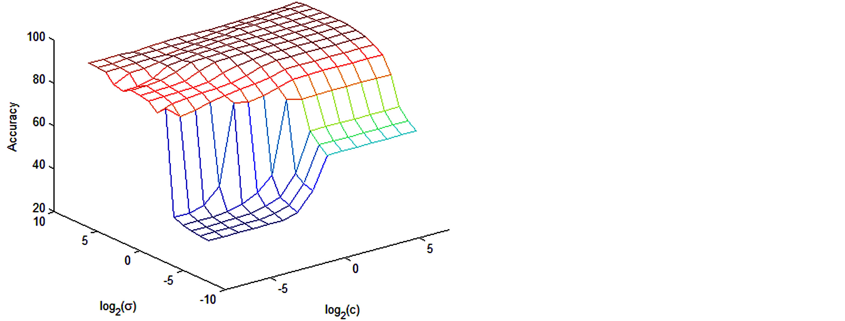
Figure 1. Tuning radial basis kernel.
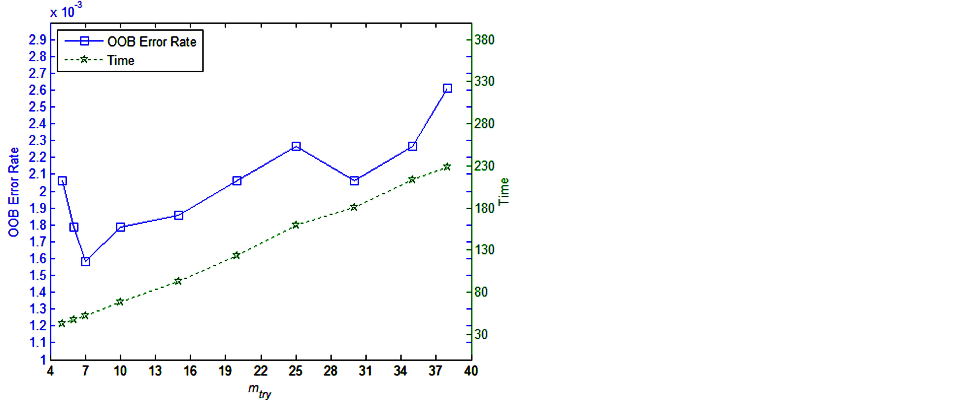
Figure 2. OOB error rates and required time to train the random forest as the number of mtry increases.
error reaches zero; instead they converge to their “asymptotic” values, which is close to their minimum. In this work, we have used ntree = 100.
To determine the minimum node size, we have used TrainSet for training and compared the OOB error rate with varying the number of node size using ntree = 100 and mtry = 7, as shown in Figure 4. The plot shows that default value 1 (one) for classification gives the lowest OOB error rate.
8. Obtained Result
The final training/test phase is concerned with the development and evaluation on a test set of the final SVM
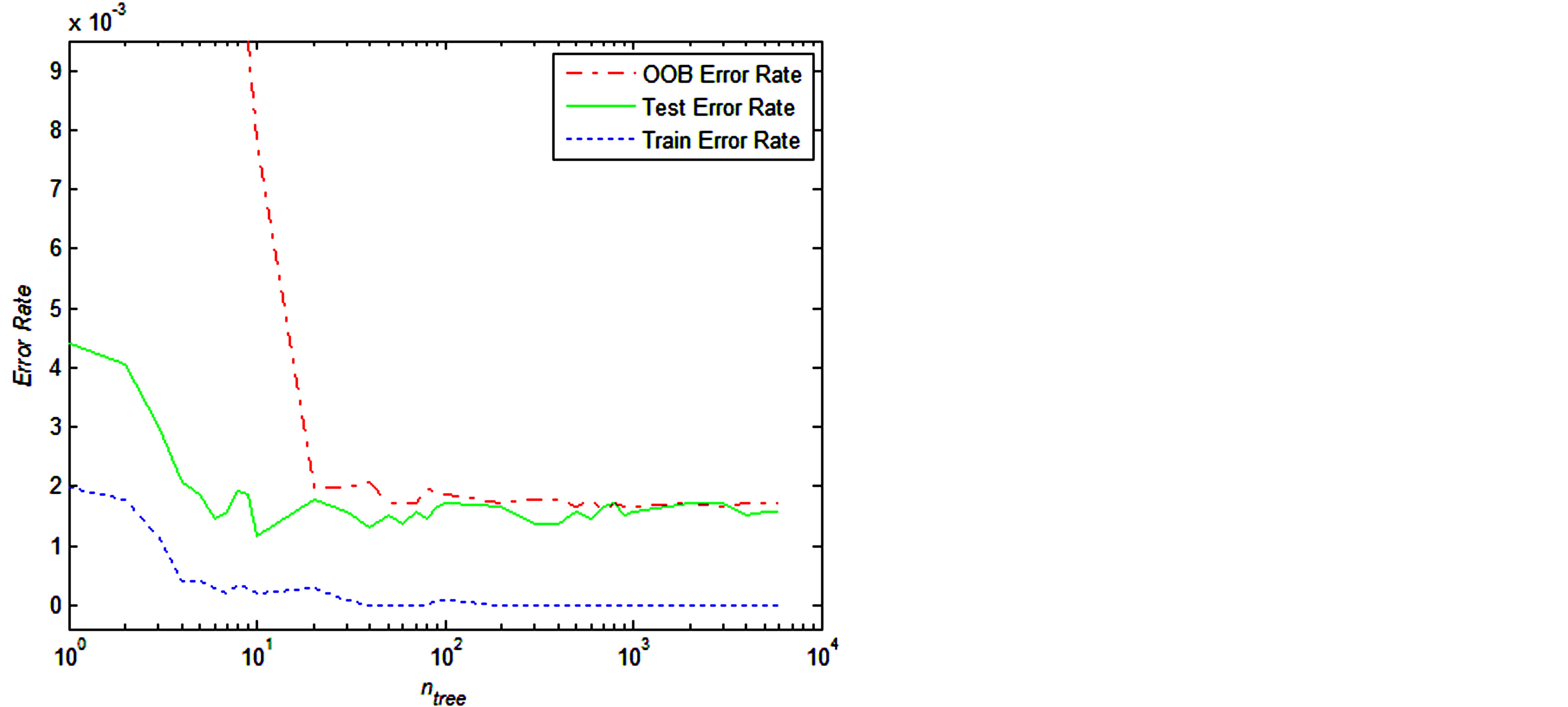
Figure 3. Comparison of training, out-of-bag, and independent test set error rates for random forest as the number of trees increases.
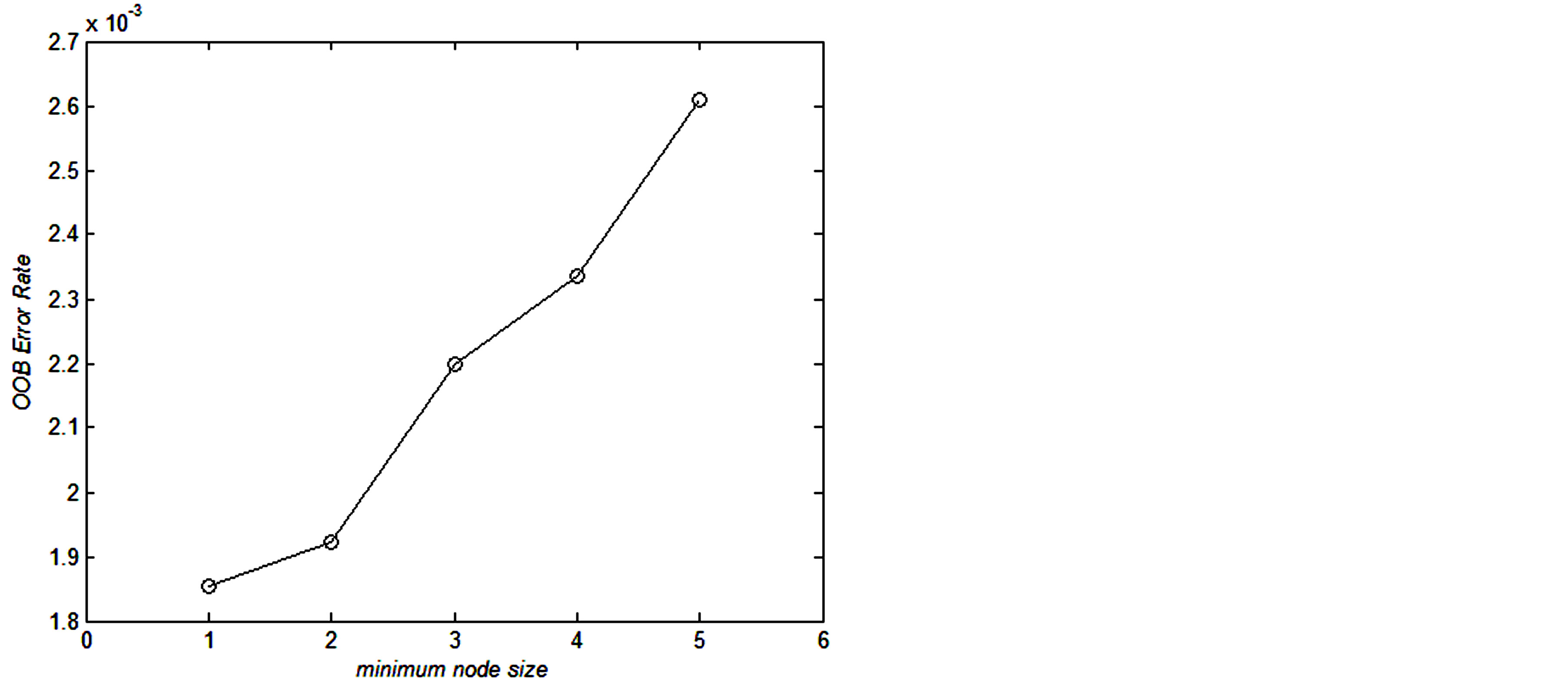
Figure 4. OOB error rates of random forest as the number of minimum node size increases.
or RF model created based on the optimal hyper-parameters set found so far in the model selection phase [17]. After finding the parameter, we have built the model using the whole train dataset (KDD99Train+) for each of the classifier (SVM and RF) and finally we have tested the model using the test dataset (KDD99Test+). The training and testing results are given in Table 5 according to the classification accuracy. From the results it is observed that the test accuracy for SVM is better than RF classifier.
For the test case, the confusion matrix for each of the classifier is given in Tables 6 and 7 respectively. Going into more detail of the confusion matrix, it can be seen that RF performs better on probing attack detection and SVM performs well on Dos, R2L, and U2R detection.
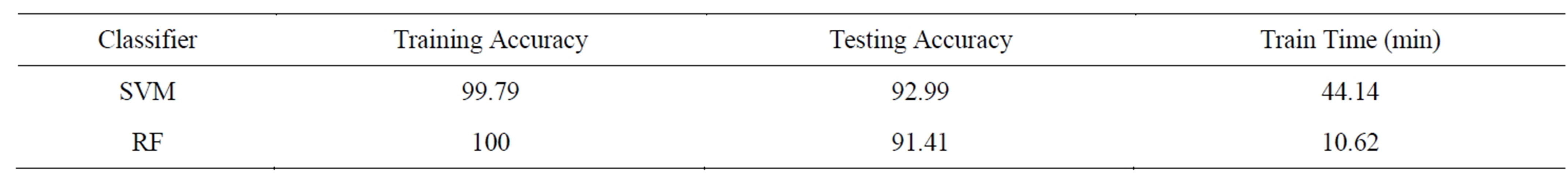
Table 5. Training and testing accuracy.
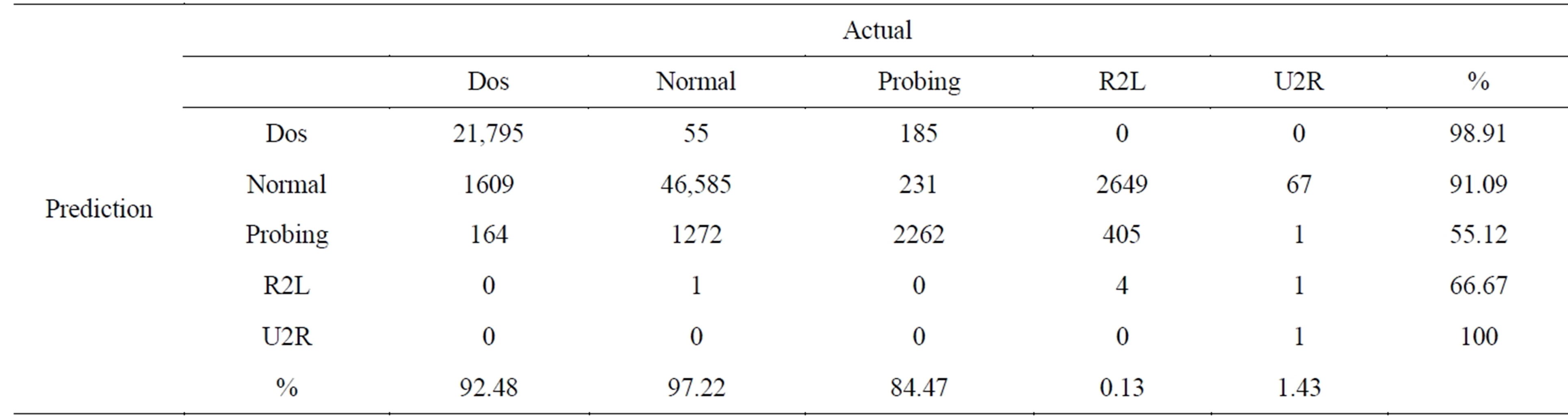
Table 6. Confusion matrix for random forest.
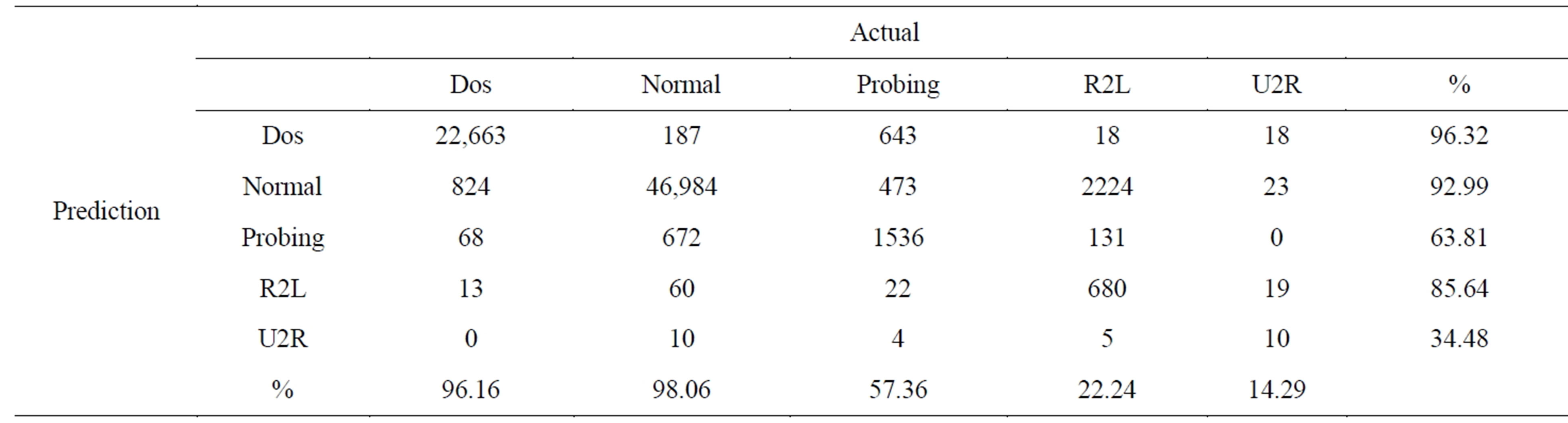
Table 7. Confusion matrix for radial basis kernel.
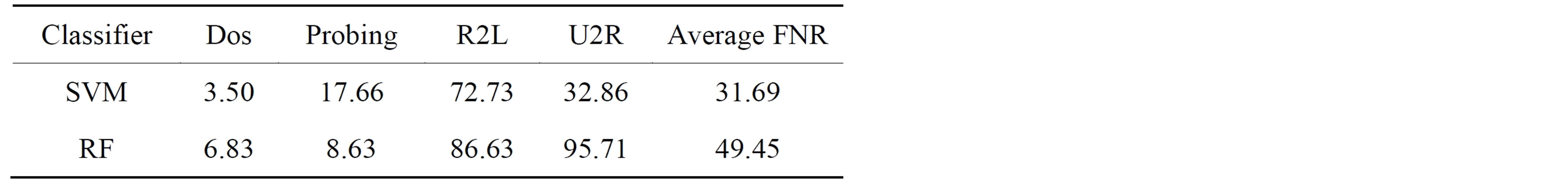
Table 8. False negative rate (FNR) for each of the attack types.
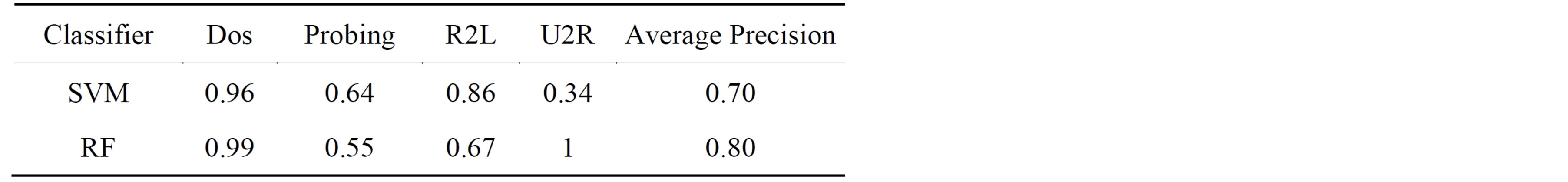
Table 9. Precision for each of the attack types.
We also considered the false negative rate and precision for each of classifier and as shown in Tables 8 and 9 respectively. The RF gives high precision and on the other hand SVM gives lower false negative rate.
9. Conclusion
In this research work, we developed two models for intrusion detection system using Support Vector Machine and Random Forest. The performances of these two approaches have been observed on the basis of their accuracy, false negative rate and precision. The results indicate that the ability of the SVM classification produces more accurate results than Random Forest and RF takes less time to train the classifier than SVM. Research in intrusion detection using SVM and RF approach is still an ongoing area due to their good performance. The findings of this paper will be very useful for future research and to use SVM and RF in a more meaningful way in order to maximize the performance rate and minimize the false negative rate.
REFERENCES
- H. G. Kayacik, A. N. Zincir-Heywood and M. I. Heywood, “Selecting Features for Intrusion Detection: A Feature Relevance Analysis on KDD 99 Benchmark,” Proceedings of the PST 2005—International Conference on Privacy, Security, and Trust, 2005, pp. 85-89.
- A. A. Olusola., A. S. Oladele and D. O. Abosede, “Analysis of KDD ’99 Intrusion Detection Dataset for Selection of Relevance Features,” Proceedings of the World Congress on Engineering and Computer Science I, San Francisco, 20-22 October 2010.
- H. Altwaijry and S. Algarny, “Bayesian Based Intrusion Detection System,” Journal of King Saud University— Computer and Information Sciences, Vol. 24, No. 1, 2012, pp. 1-6.
- O. A. Adebayo, Z. Shi, Z. Shi and O. S. Adewale, “Network Anomalous Intrusion Detection using Fuzzy-Bayes,” IFIP International Federation for Information Processing, Vol. 228, 2007, pp. 525-530.
- B. Pal and M. A. M. Hasan, “Neural Network & Genetic Algorithm Based Approach to Network Intrusion Detection & Comparative Analysis of Performance,” Proceedings of the the 15th International Conference on Computer and Information Technology, Chittagong, Bangladesh, 2012.
- S. M. Bridges and R. B. Vaughn, “Fuzzy Data Mining and Genetic Algorithms Applied To Intrusion Detection,” Proceedings of the National Information Systems Security Conference (NISSC), Baltimore, October 2000, pp. 16-19.
- M. S. Abadeh and J. Habibi, “Computer Intrusion Detection Using an Iterative Fuzzy Rule Learning Approach,” Proceedings of the IEEE International Conference on Fuzzy Systems, London, 2007, pp. 1-6.
- B. Shanmugam and N. BashahIdris, “Improved Intrusion Detection System Using Fuzzy Logic for Detecting Anamoly and Misuse Type of Attacks,” Proceedings of the International Conference of Soft Computing and Pattern Recognition, 2009, pp. 212-217.
- J. T. Yao, S. L. Zhao and L. V. Saxton, “A study on Fuzzy Intrusion Detection,” Proceedings of Data Mining, Intrusion Detection, Information Assurance, and Data Networks Security, 2005, pp. 23-30.
- Q. Wang and V. Megalooikonomou, “A Clustering Algorithm for Intrusion Detection,” Proceedings of the Conference on Data Mining, Intrusion Detection, Information Assurance, and Data Networks Security, Vol. 5812, 2005, pp. 31-38.
- V. N. Vapnik, “Statistical Learning Theory,” 1st Edition, John Wiley and Sons, New York, 1998.
- L. Breiman, “Random Forests,” Machine Learning, Vol. 45, No. 1, 2001, pp. 5-32.
- MIT Lincoln Laboratory, “DARPA Intrusion Detection Evaluation,” 2010.
- “KDD’99 Dataset,” 2010. http://kdd.ics.uci.edu/databases
- M. Bahrololum, E. Salahi and M. Khaleghi, “Anomaly Intrusion Detection Design Using Hybrid of Unsupervised and Supervised Neural Network,” International Journal of Computer Networks & Communications (IJCNC), Vol. 1, No. 2, 2009, pp. 26-33.
- H. F. Eid, A. Darwish, A. E. Hassanien and A. Abraham, “Principle Components Analysis and Support Vector Machinebased Intrusion Detection System,” 10th International Conference on Intelligent Systems Design and Applications, Cairo, November 29 2010-December 1 2010, pp. 363-367.
- M. Tavallaee, E. Bagheri, W. Lu and A. A. Ghorbani, “A Detailed Analysis of the KDD CUP 99 Data Set,” Proceedings of the 2009 IEEE Symposium on Computational Intelligence in Security and Defense Applications, Ottawa, 8-10 July 2009, pp. 1-6.
- V. N. Vapnik, “The Nature of Statistical Learning Theory,” Second Edition, Springer, New York, 1999.
- B. Scholkopf and A. J. Smola, “Learning with Kernels: Support Vector Machines, Regularization, Optimization, and Beyond,” The MIT Press Cambridge, Massachusetts London, England, 2001.
- V. Jaiganesh and P. Sumathi, “Intrusion Detection Using Kernelized Support Vector Machine with Levenbergmarquardt Learning,” International Journal of Engineering Science and Technology (IJEST), Vol. 4 No. 03, 2012, pp. 1153-1160.
- A. Ben-Hur and J. Weston, “A User’s guide to Support Vector Machines,” In: O. Carugo and F. Eisenhaber, Eds., Biological Data Mining, Springer Protocols, 2009, pp. 223-239.
- A. Mewada, P. Gedam, S. Khan and M. U. Reddy, “Network Intrusion Detection Using Multiclass Support Vector Machine,” Special Issue of IJCCT, Vol. 1, No. 2-4, 2010, pp. 172-175.
- A. Liaw and M. Wiener, “Classification and Regression by Random Forest,” R News, Vol. 2/3, 2002.
- V. Svetnik, A. Liaw, C. Tong, J. C.Culberson, R. P. Sheridan and B. P. Feuston, “Random Forest: A Classification and Regression Tool for Compound Classification and QSAR Modeling,” Journal of Chemical Information and Computer Sciences, Vol. 43, No. 6, 2003, pp. 1947- 1958.
- Y. Tang, S. Krasser, Y. He, W. Yang and D. Alperovitch, “Support Vector Machines and Random Forests Modeling for Spam Senders Behavior Analysis,” Proceedings of IEEE Global Communications Conference (IEEE GLOBECOM 2008), Computer and Communications Network Security Symposium, New Orleans, 2008, pp. 1-5.
- M. Tavallaee, E. Bagheri, W. Lu and A. A. Ghorbani, “A Detailed Analysis of the KDD CUP 99 Data Set,” Proceedings of the Second IEEE International Conference on Computational Intelligence for Security and Defense Applications, Ottawa, 2009, pp. 53-58.
- F. Kuang, W. Xu, S. Zhang, Y. Wang and K. Liu, “A Novel Approach of KPCA and SVM for Intrusion Detection,” Journal of Computational Information Systems, Vol. 8, No. 8, 2012, pp. 3237-3244.
- S. Lakhina, S. Joseph and B. Verma, “Feature Reduction using Principal Component Analysis for Effective Anomaly-Based Intrusion Detection on NSL-KDD,” International Journal of Engineering Science and Technology, Vol. 2, No. 6, 2010, pp. 1790-1799.
- J. T. Yao, S. Zhao and L. Fan, “An Enhanced Support Vector Machine Model for Intrusion Detection,” RSKT’- 06 Proceedings of the First international conference on Rough Sets and Knowledge Technology, Vol. 4062, 2006, pp. 538-543.