Journal of Water Resource and Protection
Vol.6 No.9(2014), Article
ID:47397,17
pages
DOI:10.4236/jwarp.2014.69080
Influence of Potential Evapotranspiration on the Water Balance of Sugarcane Fields in Maui, Hawaii
Javier Osorio1, Jaehak Jeong1, Katrin Bieger1, Jeff Arnold2
1Blackland Research and Extension Center, Texas A & M AgriLife Research, Temple, USA
2Grassland, Soil and Water Research Laboratory, United States Department of Agriculture, Agricultural Research Service (USDA-ARS), Temple, USA
Email: josorio@brc.tamus.edu
Copyright © 2014 by authors and Scientific Research Publishing Inc.
This work is licensed under the Creative Commons Attribution International License (CC BY).
http://creativecommons.org/licenses/by/4.0/


Received 4 March 2014; revised 2 April 2014; accepted 27 April 2014
Abstract
The year-long warm temperatures and other climatic characteristics of the Pacific Ocean Islands have made Hawaii an optimum place for growing sugarcane; however, irrigation is essential to satisfy the large water demand of sugarcane. Under the Hawaiian tropical weather, actual evapotranspiration (AET) is the primary mechanism by which water is removed from natural and agricultural systems. The Hawaiian Commercial and Sugar Company (HC&S), the largest sugarcane grower of the Hawaiian Islands, has developed a locally optimized AET equation for the purpose of water management on its 184.3 km2 sugarcane plantation on the Island of Maui. In this paper, in order to assess the influence of AET on the hydrological water balance of the HC&S’ sugarcane cropping system, the performance of the HC&S method was compared with three physically-based methods: Penman-Monteith, Priestley-Taylor, and Hargreaves, as well as, to a set of historical pan evaporation data. A Soil and Water Assessment Tool (SWAT) project was setup to estimate the water balance in two sugarcane fields: a windy lowland field and a rocky highland field on a hill slope. Under Hawaiian weather conditions, wind speed was found to be the most influential climatic parameter over potential evapotranspiration (PET); therefore, the results with both Hargreaves and Priestley-Taylor underpredicted PET by approximately 30%, presumably because these methods do not take wind speed into account. The HC&S method was demonstrated to be the most accurate PET method compared to the other commonly used PET equations, with less than 10% error. Of the annual total water supply of 3400 mm, AET accounted for 75% - 80% of the total water consumption. These findings can be used to improve the irrigation efficiency as well as other management scenarios to optimize water use on the Island of Maui.
Keywords
Evapotranspiration, Water Balance, Hydrological Modeling, Sugarcane, SWAT

1. Introduction
The year-long warm temperatures and other climatic characteristics of the Pacific Ocean Islands have made the Island of Maui an optimum place for growing sugarcane (Saccharum officinarum L.). Because of the high water demand of sugarcane, irrigation becomes one of Maui’s major constraints [1] . According to McMahon et al. [2] irrigation is essential to satisfy the large water demand of sugarcane for optimum growth and yield. In Maui, large quantities of surface and ground water from the windward side of the island are diverted by intake structures into ditches and tunnels to transport the water to the leeward plains, where the best agricultural soils are located [1] . However, mild droughts and periods of low rainfall have adversely affected the perennial streams and depleted high-level groundwater aquifers that supply Maui’s irrigation system. As water resources become limited, effective use of available water for irrigation is of concern throughout the sugarcane industry [3] .
The Hawaiian Commercial & Sugar Company (HC&S), the largest sugarcane grower of the Hawaiian Islands, has an area of 184.3 km2 under sugarcane production on the Island of Maui. The productivity of sugarcane on Maui (159.9 t∙ha−1 sugarcane yield and 24.9 t∙ha−1 sugar yield) is known to be above the national average (78.8 t∙ha−1 sugarcane yield and 9.2 t∙ha−1 sugar yield) and higher than other major sugarcane producing regions in USA like Louisiana (51.3 t∙ha−1 sugarcane yield and 6.6 t∙ha−1 sugar yield) or Texas (85.9 t∙ha−1 sugarcane yield and 10.0 t∙ha−1 sugar yield) [4] . The sugarcane cropping period is approximately 24 months. The company requires 760,000 m3∙d−1 of fresh water for irrigation, which is obtained from surface (fog drip and rainfall) and ground water sources (16 deep brackish-water wells) and is applied directly to the root zone of the sugarcane plants through a drip irrigation system.
From the hydrological perspective, actual evapotranspiration (AET) is the primary mechanism by which water is removed from the hydrologic cycle [5] -[7] . AET returns land-based water to the atmosphere through processes such as transpiration, evaporation from the plant canopy and the soil and sublimation when snow is present [8] . The rate of AET for a given environment is a function of four critical factors: soil moisture, plant type, stage of plant development, and weather conditions. In addition, the transpiration rate is influenced by soil management practices [7] [9] . McCuen [10] asserts that the most influential climatic factors on ET are temperature, relative humidity, radiation rates and wind speed.
Large AET rates in agricultural regions impact water quantity and quality [11] [12] . Accordingly, the amount of water needed for irrigation of agricultural systems is frequently calculated based on estimated AET. Underestimation of AET leads to an insufficient water supply to the crop and consequently to water stress, while overestimation of AET leads to a waste of water for irrigation. Therefore, accurate estimation of AET plays a critical role in the assessment, planning and management of water resources in general [11] . Several methods are used to estimate AET based on mass transfer, energy budget, water budget, soil moisture budget, ground-water fluctuations or meteorological variables. Each method has advantages and disadvantages; moreover, none is applicable under all conditions because of assumptions in the method or type of required data [13] . Most of the hydrological models employ the concept of potential evapotranspiration (PET) as the driving function for the calculation of AET [7] [14] [15] . PET is defined as the amount of water that would be removed from a vegetated landscape with no restrictions other than the atmospheric demand [16] , and is often measured with evaporation pans. Also, PET can be estimated using methods based on available climate data [7] [17] . Currently, a number of methods that vary in complexity and data requirements are employed for calculating PET [2] [7] [9] . Their ability to produce consistent and meaningful PET estimates depends on their assumptions, data requirements and consideration of atmospheric factors [2] [15] . HC&S has remained in the sugarcane industry for more than 100 years and during this time the company has made numerous innovations on sugarcane technology, irrigation techniques, and crop management for the sugarcane plantation on the Island of Maui. To optimize water usage for irrigation purposes, HC&S has developed a locally calibrated PET method, which is based on pan evaporation measurements and is specific to sugarcane.
The main objective of this study was to evaluate the efficiency of the HC&S irrigation system by comparing the accuracy of AET estimation by the HC&S method against three physically-based methods: Penman-Monteith, Priestley-Taylor, and Hargreaves, as well as, to a set of historical pan evaporation data and to identify an AET method that is applicable to other crops and transferable to locations with similar characteristics.
2. Data and Methods
2.1. SWAT Model
SWAT is a physically based, semi-distributed, and long-term continuous watershed scale model that runs on a daily time step to predict the impact of climate, landuse, soil type, topographic characteristics, and land management practices on hydrology, sediment, nutrients, pesticides, and bacteria in large ungauged watersheds [18] [19] . SWAT estimates PET using physically based methods that are based on historical weather variables and plant/soil available water. The methods included are Hargreaves, Priestley-Taylor, and Penman-Monteith.
Runoff is estimated by the SCS Curve Number (CN) method (SCS, 1986) or the Green & Ampt method [20] . If the Green and Ampt method is used to calculate surface runoff, the model calculates canopy storage and evaporates any readily available water present in the canopy. In contrast, the CN method lumps canopy interception, surface storage and infiltration in its initial abstraction term. After calculating runoff, SWAT calculates the amount of transpiration under ideal conditions as a function of available water in the soil. Sublimation will occur if snow is present; otherwise, the actual amount of water evaporated from the soil is calculated as a function of soil depth, water content and the above-ground biomass.
SWAT simulates the water balance according to Equation (1), which includes AET, canopy interception, plant transpiration and soil evaporation, surface runoff, and vertical water movement in the unsaturated soil zone to the ground water:
![]() (1)
(1)
where, SWi is the final soil water content (mm) in day i, SW0 is the initial soil water content (mm), i is the time (days), Ri is the amount of precipitation (mm∙day−1), Ii is the amount of daily irrigation (mm∙day−1), Qi is the amount of surface runoff (mm∙day−1), AETi is the amount of actual evapotranspiration (mm∙day−1), and PERi is the amount of water percolating through the soil profile (mm∙day−1).
2.2. PET Methods
The Penman-Monteith method [21] (Equation (2)) is a theoretically based approach that incorporates energy and aerodynamic considerations [22] . It includes a measure of the resistance to the diffusion of water vapor into the Penman’s equation, which is a radiation-aerodynamic combination equation to predict evaporation from open water, bare soil, and grass [23] :
 (2)
(2)
where: l is the latent heat flux density (MJ∙m−2kg−1), E is the depth rate evaporation (mm∙day−1), Δ is the slope of the saturation vapor pressure-temperature curve (kPa˚C−1), Hnet is the net radiation (MJ∙m−2d−1), G is the heat flux density to the ground (MJ∙m−2d−1), ρair is the air density (kg∙m−3), cp is the specific heat constant pressure (kPa∙kg−1˚C−1), ![]() is the saturation vapor pressure of air at height z (kPa), ez is the water vapor pressure of air at height z (kPa), γ is the psychometric constant (kPa˚C−1), rc is the plant canopy resistance (s∙m−1), and ra is the diffusion resistance of the air layer (aerodynamic resistance) (s∙m−1).
is the saturation vapor pressure of air at height z (kPa), ez is the water vapor pressure of air at height z (kPa), γ is the psychometric constant (kPa˚C−1), rc is the plant canopy resistance (s∙m−1), and ra is the diffusion resistance of the air layer (aerodynamic resistance) (s∙m−1).
The Priestley-Taylor method [24] (Equation (3)) is an energy-based approach. According to Jensen et al. [16] under wet conditions, evaporation from surfaces could be estimated using a simplified version of the Penman equation, in which the aerodynamic was deleted and the energy term is assumed to be a constant fraction α0 = 1.28.
 (3)
(3)
where: l is the latent heat of vaporization (MJ∙kg−1), E0 is the PET (mm∙d−1), α0 is a coefficient, Δ is the slope of the saturation vapor pressure-temperature curve (kPa˚C−1), γ is the psychometric constant (kPa˚C−1), Hnet is the net radiation (MJ∙m−2d−1), and G is the heat flux density to the ground (MJ∙m−2d−1). In semiarid conditions this equation will underestimate PET.
The Hargreaves method [25] (Equation (4)) was originally derived from eight years of cool season Alta fescue grass lysimeter data from Davis, CA. According to Hargreaves and Allen [23] the main advantage of the Hargreaves approach to the other methods is the reduced data requirement.
 (4)
(4)
where: l is the latent heat of vaporization (MJ∙kg−1), E0 is the PET (mm∙d−1), H0 is the extraterrestrial radiation (MJ∙m−2d−1), Tmax is maximum air temperature for a given day (˚C), Tmin is minimum air temperature for a given day (˚C), and Tav is the mean air temperature for a given day (˚C).
The HC&S method (Equation (5)) is specific for sugarcane and also site-specific to the central isthmus of Maui. It was developed to take into account that evapotranspiration is greatly modified by the marine surroundings and the topographic characteristics of the Island of Maui. The HC&S method to calculate PET is an empirical relationship that relates extensive pan evaporation data collected in the central isthmus of Maui [26] and locally measured meteorological parameters, such as air temperature, humidity, solar radiation and wind.
This method calculates PET by including a coefficient that multiplies the saturation vapor pressure, average actual vapor pressure, the slope of the saturation vapor pressure, a weighting function for temperature, net radiation expressed as equivalent evaporation and wind function.
 (5)
(5)
where E0 is the PET (mm∙d−1), C is a correction coefficient, Hnet is the net radiation expressed in equivalent evaporation (mm∙d−1), W is a weighting function for temperature, ![]() is the saturation vapor pressure of air at average temperature (kPa), ez is the actual water vapor pressure of the air (kPa), and Vf is a wind function.
is the saturation vapor pressure of air at average temperature (kPa), ez is the actual water vapor pressure of the air (kPa), and Vf is a wind function.
The correction coefficient (C) is calculated with a polynomial equation that includes eight coefficients and the ratio of average diurnal and nocturnal wind speed, solar radiation expressed in equivalent evaporation, and the mean wind speed. PET is multiplied by a crop coefficient (Kc) to calculate AET. To account for seasonal differences in crop growth and AET, two different crop coefficient curves are used depending on the time of planting.
3. Study Area
The study area is located on the Island of Maui, Hawaii (20˚54' latitude and 156˚26' longitude) (Figure 1) and consists of sugarcane fields (184.3 km2) that lie on elevations between sea level and 332 m. The climate of Maui is controlled primarily by topography and the position of the North Pacific anticyclone and other migratory weather systems relative to the island [11] . The climate is characterized by mild temperatures, cool and persistent trade winds, a rainy winter season from October through April, and a dry summer season from May through September [8] [27] . Solar energy and length of day are relatively uniform throughout the year and the surrounding ocean provides moist air and keeps temperatures fairly constant without extremes throughout the year [27] . Mean annual precipitation on Maui Island ranges from 7000 mm to 400 mm or less [28] . According to NOAA [29] , based on a 30-year dataset from the Kahului Station, Maui’s Central Valley, where the HC&S Co. is located, receives an average rainfall of 453 mm per year and has an average daily temperature of 24.3˚C (ranges from 19.7˚C to 29.0˚C) and an average wind velocity of 5.7 m∙s−1. Relative humidity ranges from 53% to 81%.
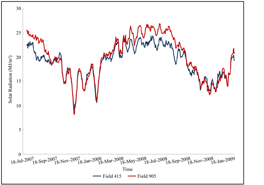
Two fields were selected for this analysis: 905 and 415. They are located in contrasting micro-climates and landscapes. Field 905 is located at a lower elevation (31.0 m a.s.l.) with a slope of 4.3%. The soil texture is classified as silt-loam and the soils are in hydrologic group B. In contrast, Field 415 is located at a higher elevation (195.4 m a.s.l.) with a slope of 6.0%. The soil texture is classified as silty-clay-loam and the soil belongs to hydrologic group C [30] . Solar radiation (Figure 2(a)), wind velocity (Figure 2(b)), average temperature (Figure 2(c)) and relative humidity (Figure 2(d)) are plotted for both fields. There are no significant differences between fields 415 and 905 with regard to average temperature (23.7˚C and 23.6˚C), relative humidity (0.71 and 0.68), and solar radiation (18.9 and 20.0 MJ∙m−2). However, wind velocity shows significant differences between both fields (2.5 and 5.8 m∙s−1), with higher speeds found in Field 905. Relative differences for average temperature, relative humidity and solar radiation are: 2.8%, 5.9% and 2.2% respectively, while the relative difference for wind velocity is 54.9%. Temperatures and humidity are higher at Field 415 while solar radiation and wind speed
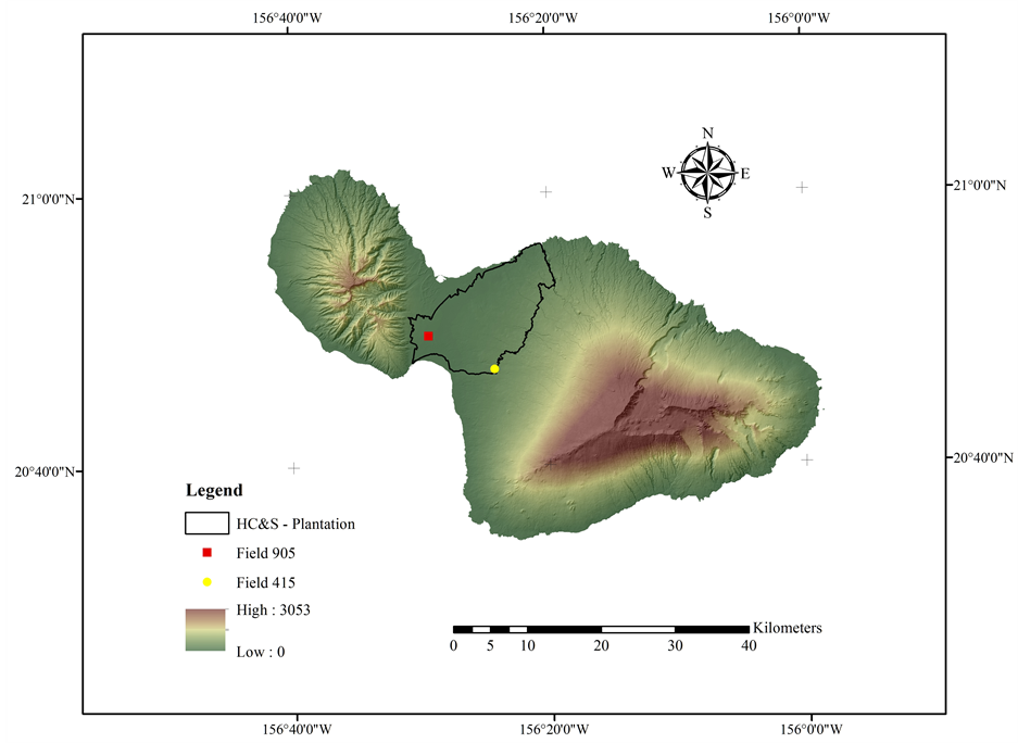
Figure 1. Location of the HC&S plantation on the Island of Maui, Hawaii.
are higher at Field 905. On Field 415, the sugarcane was planted in winter, while on Field 905 the crop was established in summer.
3.1. Input Data and Model Setup
The Digital Elevation Model (DEM) with a resolution of 10 m (1/3 arc-second) was acquired from the National Elevation Dataset (NED) [31] (available at http://viewer.nationalmap.gov/viewer/). Detailed soil map and properties for the study area were obtained from the Natural Resources Conservation Service (NRCS)—Soil Survey Geographic (SSURGO) Database (Soil Survey Staff NRCS-USDA, 2011) available at http://soildatamart.nrcs.usda.gov. The soils in the HC&S plantation area are classified as Mollisols (46.3%), Andisols (15.4%) and Aridisols (15.1%), Oxisols (10.4%), Entisols (6.0%), Inceptisols (4.2%) and Ultisols (2.3%). The landuse map and related information were obtained from the United States Geological Service (USGS) Land Cover Institute (LCI) [32] available at the USGS-Seamless Data Warehouse (http://seamless.usgs.gov/) with a resolution of 30 m (1 arc-second). The agricultural land was characterized as a 2-year sugarcane crop. The ArcGIS Interface for SWAT2012 was used to delineate the boundaries of 701 sugarcane plots, defining each plot as an individual Hydrologic Response Unit (HRUs) with sizes ranging from 1.4 to 166.0 ha.
The model uses a 12-year dataset of daily climatic records from 39 rain gauges and 12 weather stations maintained by HC&S. The climatic variables included are precipitation, minimum and maximum temperature, relative humidity, solar radiation and wind speed. Missing values in the dataset were simulated by the model’s builtin weather generator based on the weather statistics of the study area. HC&S applies water to the sugarcane fields through a drip irrigation system. The company maintains records of the applied volumes of water and the date of irrigation for each individual field. The SWAT model source code was modified to automatically read a database of dates and measured volumes of water applied to each field for irrigation purposes. For this study, historical daily irrigation data from 2003 to 2012 were acquired from the HC&S archive. Based on data availa-
 (a)
(a)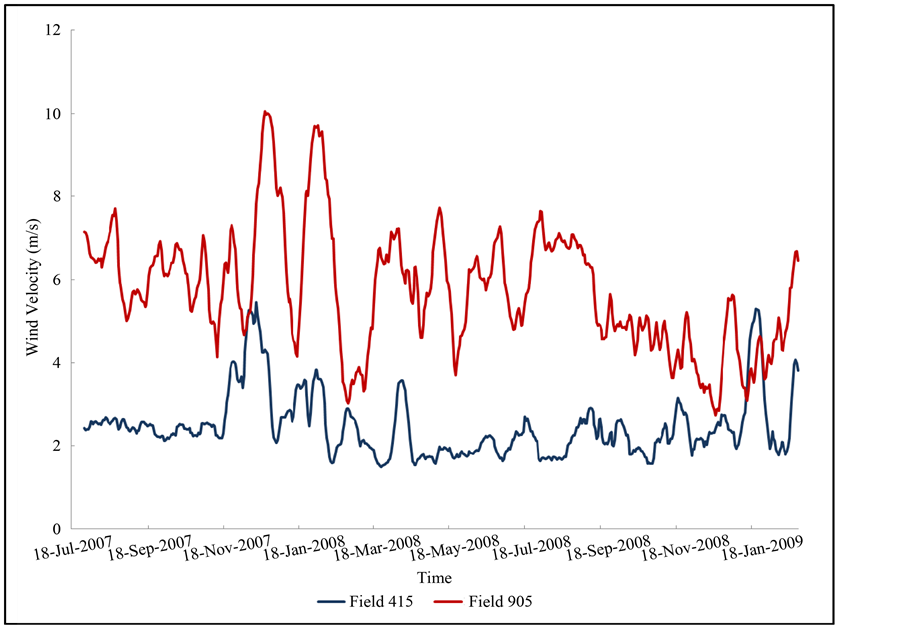 (b)
(b)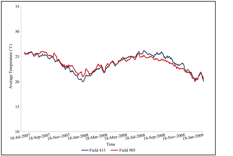 (c)
(c)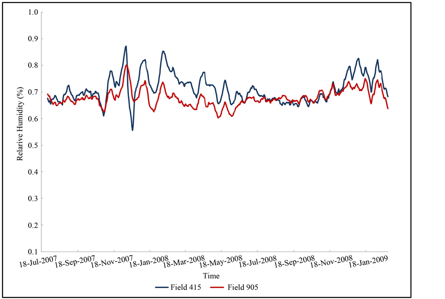 (d)
(d)
Figure 2. Measured climatic variables for the crop period at fields 415 and 905: (a) Solar radiation (MJ∙m−2); (b) Wind velocity (m∙s−1); (c) Average temperature (˚C); and (d) Relative humidity (%).
bility, the simulation period was set up for 10 years (2003-2012) with the first year of simulation set as a spinup period. However, the analysis of model output was performed for the crop period that comprises the years 2007 through 2009.
The water balance analysis was done evaluating surface runoff, percolation, lateral flow, precipitation, irrigation and available soil water. In addition, the relative difference between the predicted average annual PET and measured pan evaporation was calculated for the four PET methods included in this study. Measurements of pan evaporation in Hawaii began in 1894 and include intermittent observations for over 200 sites [26] . Most sites had standard, galvanized Class A pans on the surface, but many were later replaced with stainless steel pans to avoid corrosion and set on 1.52 m (equivalent to 5 ft) high platforms. The pan evaporation data used in this study ware corrected to account for differences due to height and pan material. A total of 12 galvanized Class A pans provided a data set with accumulated monthly and annual evaporation for the interval between 1963 and 1983. There were no Pan A measurements at the fields evaluated in this study; therefore, the closest available information to each field was used for comparison.
3.2. Crop Yield Calibration
The water balance in agricultural watersheds is influenced by crop production [33] . Crop dry matter production in Hawaii depends on the amount of water available from rainfall and irrigation [34] . The yield of a given crop can generally be described as a function of cumulative AET [35] . The AET has been shown to be directly related to dry biomass production when factors such as fertility, sunshine, temperature, and soil moisture are not limiting [36] . The following SWAT parameters were used for the purpose of manually calibrating crop yield: the soil evaporation compensation coefficient (ESCO), the plant uptake compensation factor (EPCO) and the biomassenergy ratio (BIO_E) (kg·ha−1/MJ·m−2). ESCO adjusts the depth distribution of soil evaporation to meet soil evaporative demand and varies between 0.01 and 1.0. As the value of ESCO is reduced, the model is able to evaporate more water from deeper layers in the soil profile. EPCO compensates water between soil horizons to meet the potential water uptake and ranges from 0.01 to 1.0. As EPCO approaches 1.0, the model allows more of the water uptake demand to be met by lower layers in the soil. BIO_E is the amount of dry biomass produced per unit intercepted solar radiation in ambient CO2 and varies between 10 and 90. The greater BIO_E, the greater the potential increase in total plant biomass on a given day. An important parameter governing crop growth in SWAT is the leaf area index (LAI), which controls the amount of light intercepted by the plant and converted to biomass. Also, LAI is used to calculate AET. When LAI is larger than 3, SWAT assumes that AET equals PET. To calibrate the LAI curve calculated by SWAT, it was compared to the crop coefficient curve used by the HC&S method. To evaluate crop yields simulated by SWAT, they were compared to field measurements of crop yield obtained between 2003 and 2012.
4. Results
4.1. Calibration of Sugarcane Yield
While the default values for the parameters ESCO and EPCO of 0.95 and 1.0 and BIO_E (kg∙ha−1/MJ∙m−2) of 25 were used to initialize the model; the calibrated values for the same parameters were 0.5, 0.98, and 22.5, respectively. By calibrating BIO_E, the leaf area index curve break point (LAI = 3) was adjusted to the break point of the crop coefficient (Kc = 1) used by HC&S for both winter (Field 415) and summer (Field 905) planting (Figure 3(a) and Figure 3(b)). Simulated average crop yields for the 2003-2012 period of time are 71.7 t∙ha−1 (±11.3 t∙ha−1) and 77.7 t∙ha−1 (±12.0), for fields 415 and 905 respectively. Field measurements of crop yield for fields 415 and 905 provide an average value of 71.3 t∙ha−1 (±7.7 t∙ha−1) and 77.3 t∙ha−1 (±10.0 t∙ha−1), respectively. Predicted crop yields were not different from measured values for both fields (relative differences lower than 1%). No other goodness-of-fit metrics were used in this study due to limitations in measured data. Successful calibration of crop yield guaranteed that AET was adequately represented by the model and varied accordingly as a function of climatic variables and crop development. In addition, properly predicted AET assured appropriate partitioning of the remaining components of the water budget (Figure 3(a), Figure 3(b)).
4.2. Potential Evapotranspiration (PET)
The PET values estimated by the four methods shared a concurrent spatial pattern and temporal trend. Calcula-
 (a)
(a)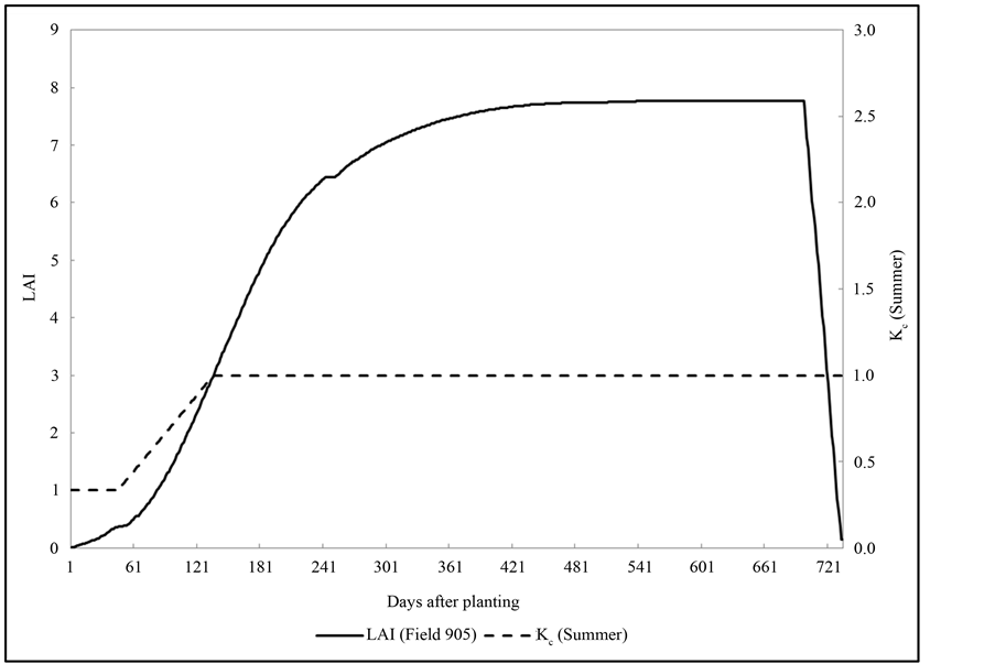 (b)
(b)
Figure 3. Leaf area index (LAI) compared to crop coefficient (Kc) for (a) the summer crop on field 415 and (b) the winter crop on field 905.
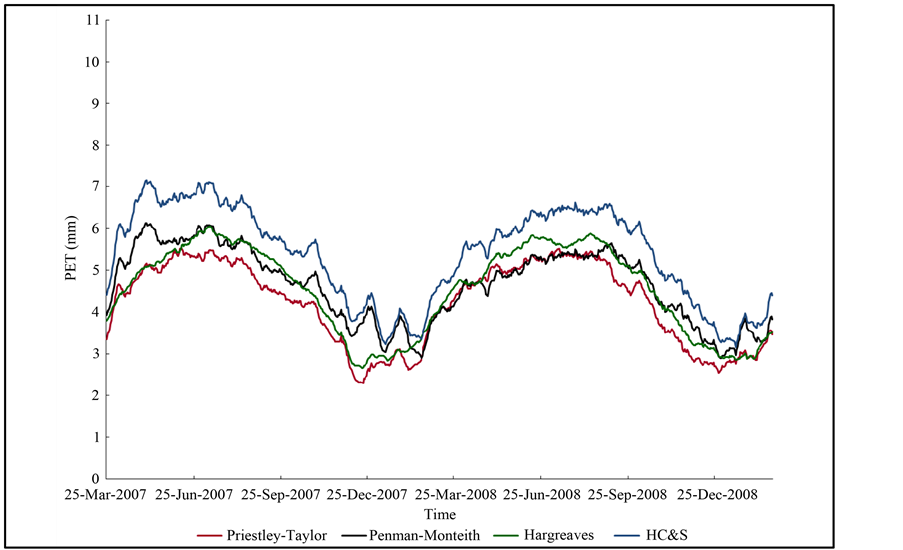
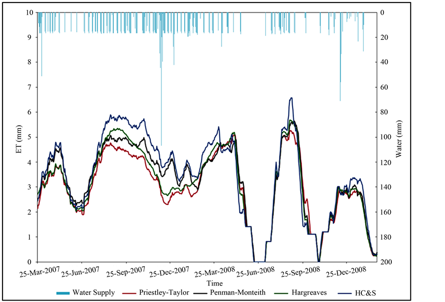
tion of PET with Hargreaves or Priestley-Taylor produced values that strongly deviate from the HC&S and Penman-Monteith methods. These differences are more obvious during the summer months (May to October) than during the winter months (November to April). A comparison of daily series of PET obtained with different methods is presented in Figure 4(a), Figure 4(b). At Field 415, predicted annual PET is 1964.3 mm using the
 (a)
(a)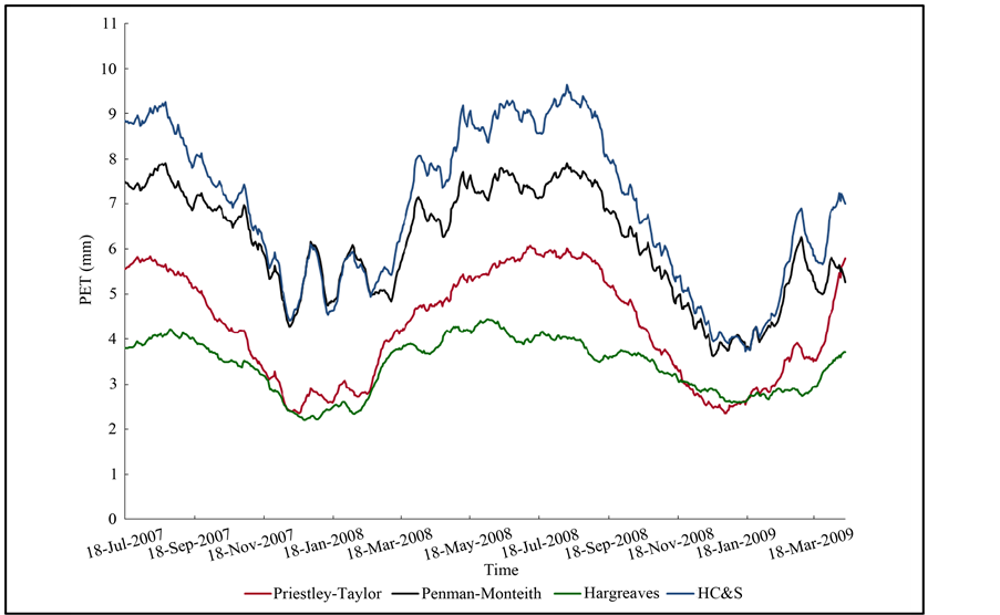 (b)
(b)
Figure 4. Comparison of PET calculated by the four tested methods at Fields 415 (a) and 905 (b).
HC&S method, 1693.6 mm using Penman-Monteith, 1656.5 mm using Hargreaves, and 1542.2 mm using Priestley-Taylor. At the nearest site, measured pan evaporation has an average of 2265.5 mm ± 193.3 mm. The relative errors of the simulated values with respect to pan measurements are 13.3% for the HC&S method, 25.2% for Penman-Monteith, 26.9% for Hargreaves, and 31.9% for Priestley-Taylor. At Field 905, PET calculated using the HC&S, Penman-Monteith, Priestley-Taylor, and Hargreaves methods is 2320 mm, 2059.5 mm, 1447.2 mm, and 1157.9 mm, respectively. Measured pan evaporation nearest to Field 905 has an average of 2466.55 mm ± 244.5 mm. The relative errors are 5.9%, 16.5% mm, 41.3%, and 53.1% for the HC&S, Penman-Monteith, Priestley-Taylor, and Hargreaves methods, respectively.
4.3. Actual Evapotranspiration (AET)
SWAT calculates AET based on LAI or the crop coefficient method until LAI equals 3. After that, the crop is assumed to be fully developed and the model assumes that all PET is partitioned to plant water uptake and soil evaporation is assumed to be negligible. However, regardless of the crop stage, soil moisture is the limiting factor that determines the volume of water that is evaporated in a given day. This critical process is well represented in SWAT. Figure 5 shows the effect of shorter periods of low soil water contents, which reduce the AET rate to the minimum possible. A comparison of AET methods for both fields 415 and Field 905 are presented in Figure 5(a), Figure 5(b). Annual AET values predicted by SWAT range from 1081 mm to 1544 mm.
Table 1(a) and Table 1(b) show the average AET values and the corresponding standard deviations for four different crop stages. The crop cycle for sugarcane was divided into growth stages defined by the break points of the crop coefficient curves used by HC&S for winter and summer plantings. At Field 415 the highest average values of AET were found during the germination and establishment phase for all methods, while at Field 905 the highest average AET values correspond to the grand growth phase. One reason for this behavior is that both fields experienced several days of water stress during the grand growth phase, which caused AET to stop completely.
In addition, the ratio between AET estimated by the Penman-Monteith and HC&S methods were calculated for the period of time where PET is all partitioned to plant uptake and no soil evaporation occurs (grand growth phase). The ratio AET/PET can be interpreted as being equivalent to the pan coefficients, which are ratios of PET to pan evaporation for a given vegetative land cover. The calculated ratios are 1.16 ± 0.11 and 1.14 ± 0.12 for fields 415 and 905, respectively. The ratios found in this study are consistent with reported coefficients for sugarcane fields under Hawaiian conditions. USGS [37] used a sugarcane pan coefficient of 1.18 during the middle stage of growth. Reported by McMahon et al. [2] , sugarcane can have a pan coefficient as high as 1.2.
4.4. Water Balance
For hydrologic studies, the major purpose of estimating AET is to determine actual water that will be lost from the system (Figure 6). The SWAT simulated water balance for the crop period (2007-2009) is shown in Table2 The study site at Field 415 receives a total of 3149 mm (686 mm precipitation + 2463 mm irrigation). Field 905 receives a total of 2079 mm (675 mm precipitation + 2863 mm irrigation). For both fields, precipitation has a very small contribution to the water budget (27.8% and 23.4%). Most of the water supply was provided by irrigation (72.2% and 76.6%). While runoff and lateral flow explain between 2.4% to 5.1% of the water balance, AET and percolation account for 94.9% to 97.6% of the water balance calculated with the HC&S method. According to the four applied methods Priestley-Taylor, Penman-Monteith, Hargreaves, and HC&S, AET accounts for 66%, 71%, 69%, and 76% and for 67%, 79%, 58%, and 81% of the total water supply at Field 415 and Field 905, respectively. The relative contribution of the runoff is very small for both fields (0.4% to 4.3%). Lateral flow also shows little variation among different methods (7.8% - 16.4%). The proportions of percolated water represent 26.5%, 24.4%, 32.1% and 16.9% of the water supply calculated with the Priestley-Taylor, PenmanMonteith, Hargreaves, and HC&S methods respectively.
5. Discussion
Comparison of the results of PET estimates using the four methods facilitated the identification of the most suitable method given a specific level of data availability and considering the specific characteristics of the growing environment. The Hargreaves method, which relies only on air temperature, failed to represent refer-
 (a)
(a)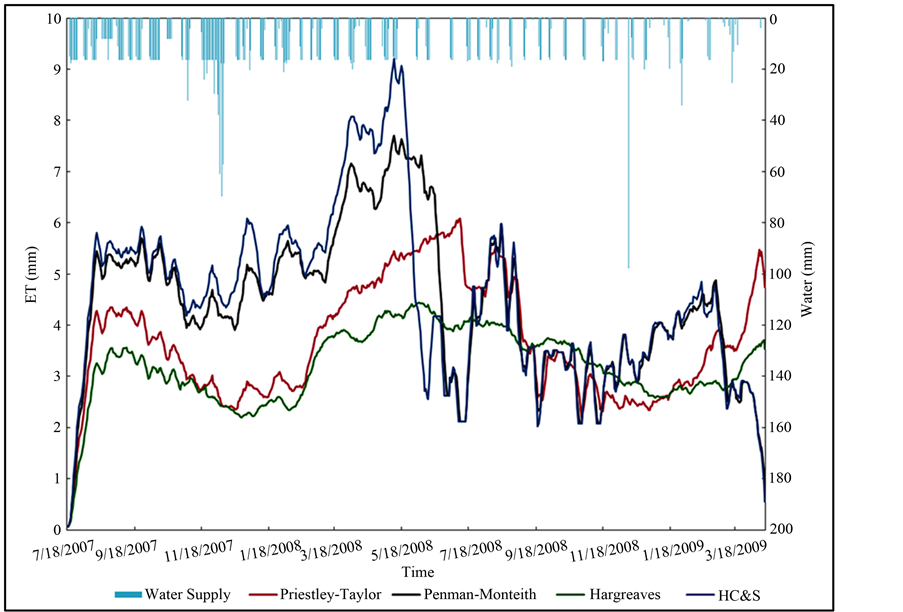 (b)
(b)
Figure 5. Comparison of actual evapotranspiration on Fields 415 (a) and 905 (b).

Table 1. Average and standard deviation of evapotranspiration by method and crop stage expressed in mm∙day−1 for Fields 415 (a) and 905 (b).
(a)
(b)
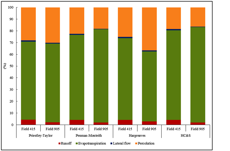
Figure 6. Water balance for Fields 415 and 905 expressed in percent of water supply.
Table 2. Water balance for Fields 415 (a) and 905 (b) expressed in mm of water. Results of the 2-year crop period.
(a)
(b)
ence evapotranspiration in irrigated regions of Maui under windy conditions. In that regard, Hargreaves and Allen [23] stated that daily estimates by the Hargreaves equation are subject to error because of the influence of the temperature range caused by large variations in wind speed. Both Hargreaves and Priestley-Taylor methods produced predictions that tended to be smaller than those predicted by the Penman-Monteith and HC&S methods. Dingman [8] concluded that temperature is not a reliable indicator of sunlight and generally is a poor predictor of pan evaporation because air temperature in Hawaii is greatly modified by the marine surroundings. Under the conditions of the study site, whenever soil water content is not the limiting factor, differences in wind velocity account for most of the variation in PET calculated with different methods. In general, PET methods, that require wind and especially humidity data, such as Penman-Monteith and HC&S, will simulate windy and humid conditions more accurately [14] [38] . The observed trends of AET as a function of crop growth stage failed to match the trends reported in other publications in which AET rises from germination phase through tillering and reaches the maximum value at the grand growth phase to then decline during the ripening phase. For instance, Freire [39] reported AET values of 3.0 mm∙day−1 for the germination phase, 3.8 mm∙day−1 for tillering phase, 5.1 mm∙day−1 for the grand growth period, and 3.1 mm∙day−1 for the ripening phase. One reason for this result could be water stress. Sugarcane at both fields had to endure a lack of rainfall and irrigation for several days at late states of the crop development. As reported, AET in sugarcane fields is highly variable largely due to local climatic conditions, hydrologic settings, and the type of production systems. However, predicted AET made by SWAT for the entire crop cycle with Penman-Monteith and HC&S methods in two different field conditions compared well to reported measured data of AET that ranges between 2.33 - 5.70 mm∙day−1 [39] -[42] .
Using the HC&S method, the proportion of percolated water (16.3% - 18.5%) compares reasonable well to 19% and 34% of recharge found as a proportion of the total water input by Izuka et al. [43] and Shade [44] . In addition, AET proportions calculated with the HC&S method (76.4% - 81.3%) are also supported by the comparisons made with measured Pan A evaporation datasets. Accordingly, it can be assumed that SWAT properly represents the system under analysis when using the HC&S method to account for AET. HC&S managers use their own modified ET equation to plan irrigation. In both fields (415 and 905), the amounts of irrigation (2463.2 mm and 2896.9 mm), i.e. the water supply, and AET (2403.4 mm and 2896.9 mm), i.e. the demand, are similar.
6. Conclusions
Considering the important role that evapotranspiration plays in the water cycle, the appropriate selection of the PET method to estimate AET is of great importance. Commonly, the PET method is selected based on the availability of climatic datasets to feed the models. The lack of climatic variables limits the use of physically sound PET approaches. However, the selection of the PET method should rather be taken based on site characteristics; the use of a PET method that takes into account the dominant climatic variables is highly recommended. By ignoring the dominant weather factor, predicted PET can be meaningless and likely not representative of the environmental conditions that need to be assessed. Based on the results of this study, the HC&S method appropriately represents the specific climatic and environmental conditions of the central valley in Maui, in which HC&S sugarcane plantations are located. However because the HC&S method was developed for very specific conditions, the Penman-Monteith method is recommended for other parts of the Hawaiian Islands, where climatic conditions are dominated by wind characteristics. In order to represent local conditions, PET during the grand growth phase of sugarcane should be calculated multiplying the Penman-Monteith PET by a coefficient that ranges between 1.14 and 1.16.
The present study assessed the influences of PET methods on the water balance of sugarcane cropping system in the Hawaiian Island of Maui. The results suggests that the proportions of ET, percolated water, lateral flow and runoff compare reasonably well with results reported in other studies performed on the Island of Maui. Accordingly, the HC&S Company allocates water for irrigation based on an appropriate estimation of AET. However, additional work should be done to analyze the entire system that includes water collection from the ditch system (including bypass water), analysis of ground water recharge and pumping system and the water budget for the entire island.
Acknowledgements
This study was funded by the US Department of Navy, Office of Naval Research & USDA-ARS Bioenergy Project in Hawaii. The authors are grateful to Mae Nakahata from HC&S for providing research access and assistance and to the anonymous reviewers for their valuable suggestions to improve the paper.
References
- Grubert, E. (2011) Freshwater on the Island of Maui: System Interactions, Supply, and Demand. Master’s Thesis, Environmental Water Resource Engineering, University of Texas at Austin, Austin.
- McMahon, T.A., Peel, M.C., Lowe, L., Srikanthan, R. and McVicar, T.R. (2012) Estimating Actual, Potential, Reference Crop and Pan Evaporation Using Standard Meteorological Data: A Pragmatic Synthesis. Hydrology and Earth System Sciences, 9, 11829-11910. http://dx.doi.org/10.5194/hessd-9-11829-2012
- Lloyd, B.R., Davidson, J.R. and Hogg, H.C. (1972) Estimating the Productivity of Irrigation Water for Sugarcane Production in Hawaii. Economic Research Service Technical Report No. 56, USDA—Natural Resource Economics Division, 72.
- National Agricultural Statistics Service (NASS) (2013) National Statistics for Sugarcane. http://www.nass.usda.gov
- Baumgartner, A. and Reichel, E. (1975) The World Water Balance. R. Oldenbourg-Verlag, Munchen, Wien, 1-179.
- Irmak, S., Howell, T.A., Allen, R.G., Payero, J.O. and Martin, D.L. (2005) Standardized ASCE Penman-Monteith: Impact of Sum-Of-Hourly vs. 24-Hour Timestep Computations at Reference Weather Station Sites. Transactions of the ASAE, 48, 1063-1077. http://dx.doi.org/10.13031/2013.18517
- Wang, X., Melesse, A.M. and Yang, W. (2006) Influences of Potential Evapotranspiration Estimation Methods on Swat’s Hydrologic Simulation in a Northwestern Minnesota Watershed. Transactions of the ASABE, 49, 1755-1772.http://dx.doi.org/10.13031/2013.22297
- Dingman, S.L. (1994) Physical Hydrology. Macmillan College Publishing Company, New York, 575.
- Allen, R.G., Pereira, L.S., Raes, D. and Smith, M. (1998) Crop Evapotranspiration: Guidelines for Computing Crop Water Requirements. FAO Irrigation and Drainage Paper 566, UN-FAO, Rome.
- McCuen, R.H. (1998) Hydrologic Analysis and Design. 2nd Edition, Prentice-Hall, Upper Saddle River.
- Giambelluca, T.W. and Nullet, D. (1992) Evaporation at High Elevations in Hawaii. Journal of Hydrology, 136, 219-235. http://dx.doi.org/10.1016/0022-1694(92)90012-K
- Farahani, H.J., Howell, T.A., Shuttleworth, W.J. and Bausch, W.C. (2007) Evapotranspiration: Progress in Measurement and Modeling in Agriculture. Transaction of the ASABE, 50, 1627-1638. http://dx.doi.org/10.13031/2013.23965
- Shih, S.F. (1987) Using Crop Yield and Evapotranspiration Relations for Regional Water Requirement Estimation. Water Resources Bulletin—American Water Resources Association, 23, 435-442.
- Gracel, B. and Quickl, B. (1998) A Comparison of Methods for the Calculation of Potential Evapotranspiration under the Windy Semi-Arid Conditions of Southern Alberta. Canadian Research Hydrology, 13, 9-19.
- Blumenstock, D.I. and Price, S. (1967) Climate of Hawaii. In: Climates of the States, No. 60-51, Climatography of the United States, US Department of Commerce, Washington DC.
- Jensen, M.E., Burman, R.D. and Allen, R.G. (1990) Evapotranspiration and Irrigation Water Requirements. American Society of Civil Engineers Manual and Reports on Engineering Practice No. 70, New York, 360.
- Bezuidenhout, C.N., Lecler, N.L., Gers, C. and Lyne, P.W.L. (2006) Regional Based Estimates of Water Use for Commercial Sugarcane in South Africa. Water South Africa, 32, 219-222.
- Arnold, J.G. and Fohrer, N. (2005) SWAT2000: Current Capabilities and Research Opportunities in Applied Watershed Modeling. Hydrolocical Processes, 19, 563-572. http://dx.doi.org/10.1002/hyp.5611
- Gassman, P.W., Reyes, M., Green, C.H. and Arnold, J.G. (2007) The Soil and Water Assessment Tool: Historical Development, Applications, and Future Directions. Transactions of the ASABE, 50, 1211-1250.http://dx.doi.org/10.13031/2013.23637
- Green, W.H. and Ampt, G.A. (1911) Studies on Soil Physics, Part 1, the Flow of Air and Water through Soils. Journal of Agricultural Science, 4, 11-24.
- Monteith, J.L. (1965) Evaporation and the Environment. 19th Symposia of the Society for Experimental Biology, 19, 205-234.
- Sumner, D.M. and Jacobs, J.M. (2005) Utility of Penman-Monteith, Priestley-Taylor, Reference Evapotranspiration, and Pan Evaporation Methods to Estimate Pasture Evapotranspiration. Journal of Hydrology, 308, 81-104.http://dx.doi.org/10.1016/j.jhydrol.2004.10.023
- Hargreaves, G.H. (1975) Moisture Availability and Crop Production. Transactions of the ASAE, 18, 980-984.http://dx.doi.org/10.13031/2013.36722
- Priestley, C.H.B. and Taylor, R.J. (1972) On the Assessment of Surface Heat Flux and Evaporation Using Large-Scale Parameters. Monthly Weather Review, 100, 81-82.http://dx.doi.org/10.1175/1520-0493(1972)100<0081:OTAOSH>2.3.CO;2
- Hargreaves, G.H. and Allen, R.G. (2003) History and Evaluation of Hargreaves Evapotranspiration Equation. Journal of Irrigation and Drainage Engineering, 129, 53-63. http://dx.doi.org/10.1061/(ASCE)0733-9437(2003)129:1(53)
- Ekern, P.C. and Chang, J.H. (1985) Pan Evaporation: State of Hawaii, 1894-1983. Hawaii. Department of Land and Natural Resources, Division of Water and Land Development, Honolulu, Rep. R74, viii + 172.
- Sanderson, M. (1993) Prevailing Trade Winds: Weather and Climate in Hawaii. University of Hawaii Press, Honolulu, 126.
- Mink, J.F. and Lau, L.S. (2006) Hydrology of the Hawaiian Islands. University of Hawaii Press, Honolulu.
- NOAA (National Oceanic and Atmospheric Administration) (2013) Comparative Climatic Data for the United States through 2012. http://ols.nndc.noaa.gov/plolstore/plsql/olstore.prodspecific?prodnum=C00095-PUB-A0001
- Anderson, R.G. and Wang, D. (2014) Energy Budget Closure Observed in Paired Eddy Covariance Towers with Increased and Continuous Daily Turbulence. Agricultural and Forest Meteorology, 184, 204-209.http://dx.doi.org/10.1016/j.agrformet.2013.09.012
- Gesch, D.B. (2007) The National Elevation Dataset. In: Maune, D., Ed., Digital Elevation Model Technologies and Applications: The DEM User’s Manual, 2nd Edition, American Society for Photogrammetry and Remote Sensing, Bethesda, 99-118.
- Fry, J.A., Coan, M.J., Homer, C.G., Meyer, D.K. and Wickham, J.D. (2009) Completion of the National Land Cover Database (NLCD) 1992-2001 Land Cover Change Retrofit Product. US Geological Survey Open-File Report 2008-1379, 18.
- Nair, S.S., King, K.W., Witter, J.D., Sohngen, B.L. and Fausey, N.R. (2011) Importance of Crop Yield in Calibrating Watershed Water Quality Simulation Tools. JAWRA: Journal of the American Water Resource Association, 47, 1285-1297. http://dx.doi.org/10.1111/j.1752-1688.2011.00570.x
- Jones, C.A. (1980) A Review of Evapotranspiration Studies in Irrigated Sugarcane in Hawaii. Hawaiian Planters’ Record, 59, 195-214.
- Liu, W.Z., Hunsaker, D.J., Li, Y.S., Xie, X.Q. and Wall, G.W. (2002) Interrelations of Yield, Evapotranspiration, and Water Use Efficiency from Marginal Analysis of Water Production Functions. Agricultural Water Management, 56, 143-151. http://dx.doi.org/10.1016/S0378-3774(02)00011-2
- Allison, F.E., Roller, E.M. and Raney, W.A. (1985) Relationship between Evapotranspiration and Yields of Crops Grown in Lysimeters Receiving Natural Rainfall. Agronomy Journal, 50, 506-511.http://dx.doi.org/10.2134/agronj1958.00021962005000090004x
- United States Geological Service (USGS) (2007) Effects of Agricultural Land-Use Changes and Rainfall on Ground-Water Recharge in Central and West Maui, Hawaii, 1926-2004. Scientific Investigations Report 2007-5103, 69.
- Suleiman, A.A. and Hoogenboom, G. (2007) Comparison of Priestley-Taylor and FAO-56 Penman-Monteith for Daily Reference Evapotranspiration Estimation in Georgia. Journal of Irrigation and Drainage Engineering, 133, 175-182.http://dx.doi.org/10.1061/(ASCE)0733-9437(2007)133:2(175)
- Da Silva, T.G.F.F. (2009) Analise de crescimento, interacao biosfera-atmosfera e eficiencia do uso de agua da cana-deacucar irrigada no submedio do vale do Sao Francisco. TeseDoutorado—Universidade Federal de Vicosa, 194.
- Souza, E.F., Bernardo, S. and Carvalho, J.A. (1999) Funcao de producao da cana—Deacucaremrelacao a agua para tres cultivares, em Campos dos Goytacazes. Engenharia Agicola, 19, 28-42.
- Inman-Bamber, N.G. and McGlinchey, M.G. (2003) Crop Coefficients and Water-Use Estimates for Sugarcane Based on Long-Term Bowen Ratio Energy Balance Measurements. Field Crops Research, 83, 125-138.http://dx.doi.org/10.1016/S0378-4290(03)00069-8
- Santos, M.A.L. (2005) Irrigacao suplementar da cana-de-acucar (Saccharumspp.): Um modelo de analise de decisao para o Estado de Alagoas. Tese Doutorado—Escola Superior de Agricultura “Luiz de Queiroz”, Piracicaba, 101.
- Izuka, S.K., Oki, D.S. and Chen, C. (2005) Effects of Irrigation and Rainfall Reduction on Ground-Water Recharge in the Lihue Basin, Kauai, Hawaii. Scientific Investigations Report 2005-5146, US Department of the Interior, 48.
- Shade, P.J. (1999) Water Budget of East Maui, Hawaii. Water-Resources Investigations Report 98-4159, US Department of the Interior, 36.