Journal of Water Resource and Protection
Vol.6 No.2(2014), Article ID:43175,7 pages
DOI:10.4236/jwarp.2014.62014
Average Rainfall Estimation: Methods Performance Comparison in the Brazilian Semi-Arid
Civil and Environmental Engineering School, Federal University of Goiás, Goiânia, Brazil
Email: klebber.formiga@gmail.com
Copyright © 2014 Fernando D. Barbalho et al. This is an open access article distributed under the Creative Commons Attribution License, which permits unrestricted use, distribution, and reproduction in any medium, provided the original work is properly cited. In accordance of the Creative Commons Attribution License all Copyrights © 2014 are reserved for SCIRP and the owner of the intellectual property Fernando D. Barbalho et al. All Copyright © 2014 are guarded by law and by SCIRP as a guardian.
Received December 16, 2013; revised January 19, 2014; accepted February 12, 2014
Keywords:Average Rainfall; Interpolation Techniques; Multiquadric Equations; Reciprocal Distance Squared Method; Semiarid Rainfall; Thiessen’s Method
ABSTRACT
Considering the rainfall’s importance in hydrological modeling, the objective of this study was the performance comparison, in convergence terms, of techniques often used to estimate the average rainfall over an area: Thiessen Polygon (TP) Method; Reciprocal Distance Squared (RDS) Method; Kriging Method (KM) and Multiquadric Equations (ME) Method. The comparison was done indirectly, using GORE and BALANCE index to assess the convergence results from each method by increasing the rain gauges density in a region, through six scenarios. The Coremas/Mãe D’Água Watershed employed as study area, with an area of 8385 km2, is situated on Brazilian semi-arid. The results showed the TP, as RDS and ME techniques to be employed successfully to obtain the average rainfall over an area, highlighting the MEM. On the other hand, KM, using two variograms models, had an unstable behavior, pointing the prior study of data and variogram’s choice as a need to practical applying.
1. Introduction
The average rainfall over an area may be considered as the main input on watershed modeling process, especially of those which deal with surface runoff, partly because, in general, the rain is the only climatic variable that can explain fast increasing flow [1-3]. Still, several studies show that spatial variability of rainfall over the basin and their distribution pattern, as well as its interaction with the basin, have considerable effect on runoff response generated [4-7].
In this sense, despite the development of radar technology has been observed, due to the limitations and characteristics of theses specialized measurements, point measurements made by rain gauge are still required for better modeling [1,8-10]. Besides, the point measures of rain are, in many places, the only available time-series source with enough spatial density for hydrological studies, so to runoff modeling, as well as to water resources planning. Thus, the study of techniques to estimate the average rainfall, using point measures, and the distribution pattern analysis, remains indispensable.
Considering the methods used to determine the average rainfall, which vary from the simple linear combination to geostatistics techniques, it’s possible to emphasize in many studies and applications: the Thiessen Polygon (TP) Method [11,12], the Reciprocal Distance Squared (RDS) Method [13-16] the Kriging Method (KM) [5, 17-19] and the Multiquadric Equations (ME) Method [16,20-25].
Besides the mean rainfall, RDS, KM and ME also estimate a continuous surface that adjusts itself to the known rainfall values, being useful on point rainfall values determination within the basin. This particular characteristic is very useful on rainfall spatial distribution evaluation [19] and provides specialized data for robust models applied in other hydrologic process.
However, the real value of average rainfall and its distribution is still an unknown variable [1]. Thus, the direct comparison of the values obtained cannot justify an complete affirmation nor denial of one or another technique in a given case. Any application of these methods must, first, assess the complexity, data availability, the scale of the problem and the additional information desired from rain behavior in some region.
Given that, the aim of this study is the comparison of techniques to estimate the average annual rainfall over a given watershed, through the analysis of results in various scenarios of data availability, in view of the water resources planning, for long and medium term, in regions with point measures predomination of. For this, it has chosen the Coremas Mãe D’Água Watershed, located in Brazilian semi-arid (Figure 1), where the major data are found as rain gauge registries, currently provided by Brazilian Water Agency-ANA.
The semi-arid climatic aspect adds more peculiarities to water resources planning because of the high variability, in time and space, of rainfall [2]. Still, the study of monthly and annual rainfall over great areas is very relevant in water resources management for these areas, where this feature is critical. These places often suffer with extreme events, too [26], which ultimately require more flexible and accurate techniques and tools for planning, not only long and medium term, but also critical flooding scenarios of interest to managers.
2. Methods and Data
It is not possible to compare values from any method with the real one, because it is unknown. It is possible to evaluate the variability (or convergence) of some model caused for a change in availability data. Thus, even that methods remain incomparable directly, find which of them would need less spatial data to achieve results supposedly more reliable (obtained in a better data scenario), it is feasible, and so comparing them indirectly, following this line: in a favorable situation which the rain gauge density was great enough. Probably all techniques would give great results, very close to real values of mean rainfall; so, it is reasonable to believe that methods with a good convergence behavior, at first, are more reliable in a less favorable situation. [4] suggested two indices, GORE and BALANCE, to compare average rainfall values given by different data subset. On the other hand, several researches have dealt with rainfall analyses
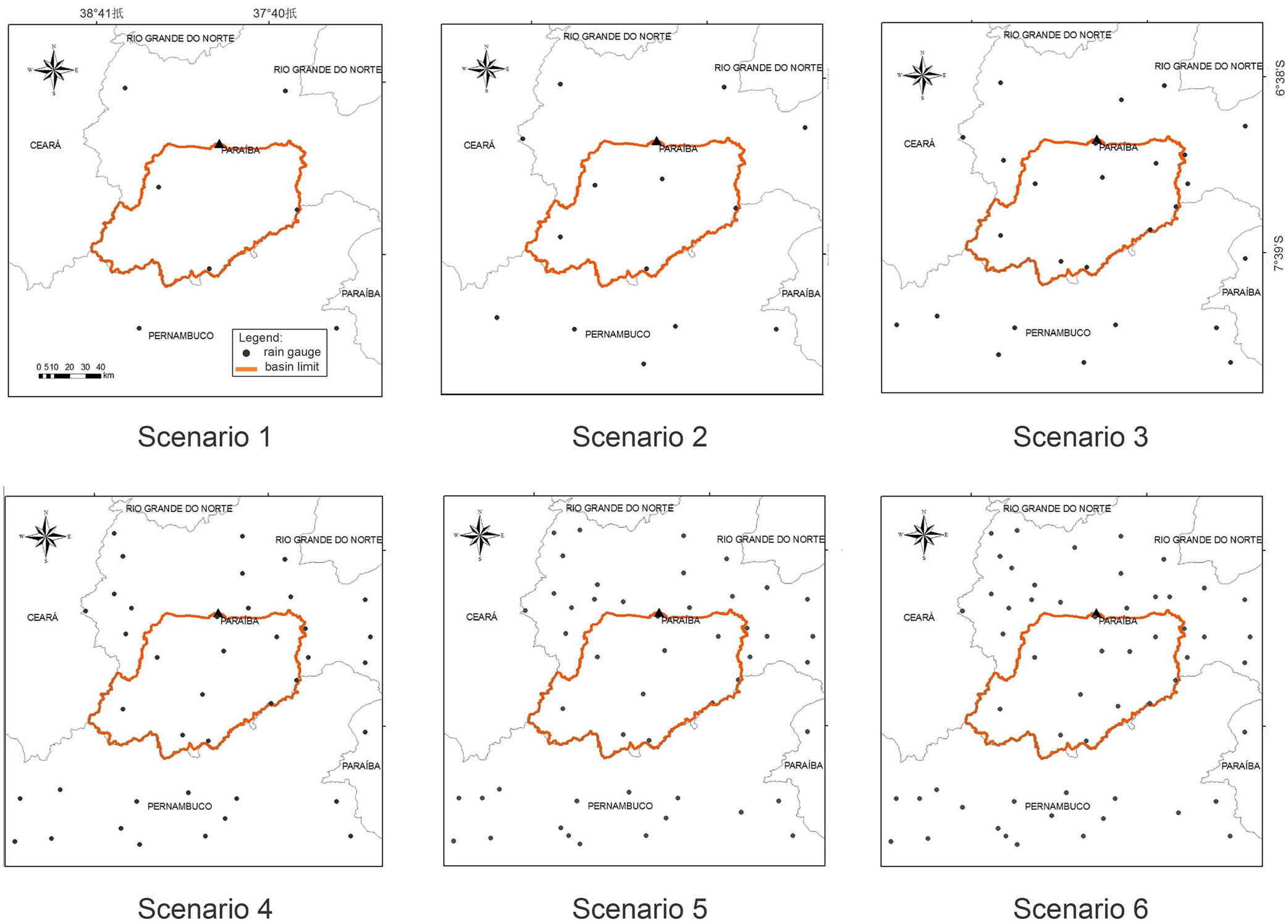
Figure 1. Scenarios utilized to compare the methods.
from the rainfall-runoff modeling perspective [1,6,7,24, 25,27]. In some cases, it was found that reducing the number of rain gauges used could improve the models accuracy, inclusive. However, in the water resources management case for great scales of time and space, it’s thought that a greater dataset will reflect in a better mean rainfall estimate and its behavior which, in some cases, is the objective of the specific study.
Thus, the previously cited methods were compared with the two indices, using five scenarios with a different spatial data density, comparing their results with those obtained from a sixth scenario with the major density available, the reference set.
For this task, 56 rain gauge stations were selected within the study area with daily records from ten consecutive years, from 1965 to 1974, being admitting just one missing year. These registers were obtained from ANA database. The gap filling was done just with the simple mean and after this the annual series for each gauge were constructed.
The Watershed of Coremas Mãe D’Água Dam was chosen as study area for this work (Figure 1). Its outfall coordinates are S 06.99˚ and W 37.96˚, resulting in a 8385 km² drainage area with 528 km of perimeter. The data search region has been defined as a rectangle, north south oriented, with an offset of 0.5˚ from basin’s limits. In this study were used the registers found for 56 stations of Paraiba and Pernambuco states. Figure 1 also shows the distribution of all stations used in each scenario.
From 56 selected stations, six scenarios were made, increasing the number of gauges until the maximum, as showed in Figure 1. The organization of them just prioritized a homogenous spatial distribution, without any preliminary evaluation, trying to ensure a random character, with no benefits to any method. Scenario 6 was taken as the reference one, because it has more spatial data available. Thus, for all calculating done, the spatial discretization taken was 0.05˚ (decimal degrees)
2.1. The Gore Method
The GORE index [4] was adapted as follows: let Pi be the real average rainfall in a given interval of time (here considering being equal to results obtained in Scenario 6, because it’s unknown in practice) and let PiE be the estimated value of rainfall for the same interval i in a given scenario, so:
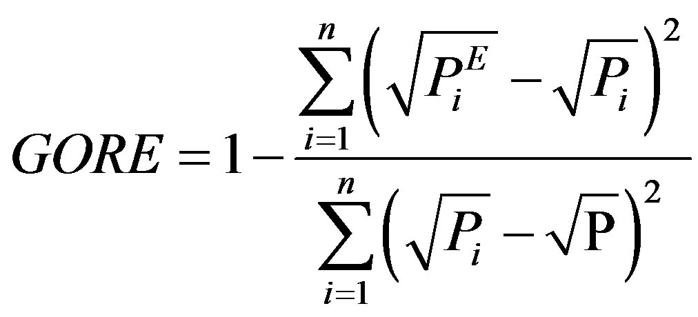 (1)
(1)
n is the time intervals number and P is the mean of Pi values for all time considered.
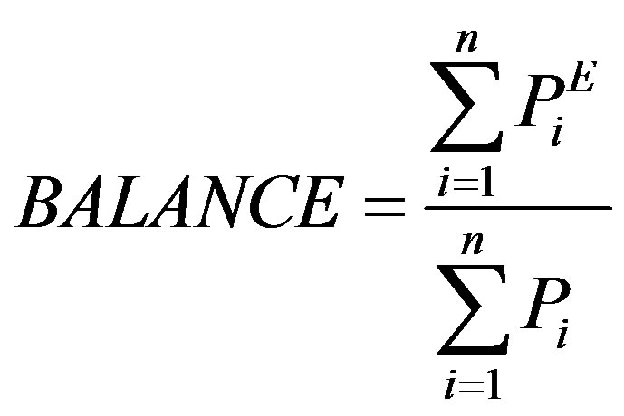 (2)
(2)
2.2. Thiessen Polygon Methods-TP
Developed by [28], TP is a simple method created to obtain the average rainfall in great areas. It’s frequently used [11,19] and its formulation consists on determining a weighted average with rainfall amount of each station, in which weights are determined according with the influence area of each station. TP is a good technique when there is a reasonable dense gauge network, otherwise mistakes may be considerable. However, according to [29], care should be taken regarding the type of precipitation being analyzed, since convective rainfall presents high temporal variability, so the measurement intervals must be compatible. Thus, [19] shows some variants of TP.
2.3. Reciprocal Distance Squared Method-RDS
[30] proposed the RDS as a tool to determine mean rainfall over a given area. This method assumes that any punctual rainfall into a given area can be estimated from the observed values, being inversely proportional to its distance to measures points. RDS may be considered as one of many interpolation techniques based on a weighting as a distance function. It’s often used in a large range of studies related with rainfall [16], being cited by [13-15] and others.
2.4. Multiquadric Equations Method-ME
The application of quadric surfaces for points data interpolation was initially developed by [20] for application in geophysical sciences. After, [21] employed it to adjust rainfall surfaces, pointing ME as a good alternative tool. It’s assumed that the real rainfall surface can be found by overlapping others individual quadric surfaces, each one starting on a known point. These surfaces may be parabolic or hyperbolic, whose adjust is smoother and, specially for conics, a more simple implementation [22], which is the formulation adopted in this study. [23] established a formal equivalence between ME and KM. [24], comparing both, chose by the use of ME for more practical with similar results. Still, [16] showed how to reduce bias of ME.
2.5. Kriging Method-KM
Based on regionalized variables concept, developed by [17], the KM consists of a set of techniques to estimate surfaces by modeling the spatial correlation structure of the variables in question. KM assumes there is a phenomena pattern, at a large scale, a local pattern and some local randomness [31]. Still, the technique has been seeing as the best linear estimator because does not present bias [18]. The determining the weight of each observation is done by an adjustment of a variogram model. The determination of the weight of each observed data was obtained by fitting a variogram model. It starts with the existing data and its position to calculate the correlations among them, then an adjustment is made upon the results obtained. Kriging formulation also allows verifying the statistical errors made [31]. However, the method presents the variogram choice problem [19]. For this work, two variograms models were tested: the KM with a Gaussian variogram (KG) and the KM with a cubic spline variogram (KCS).
3. Results and Discussion
The average rainfall on the watershed for each year and scenario (1 to 6), estimated by each method tested, is given in Table 1. On the other hand, Table 2 illustrates the results obtained for GORE and BALANCE indices
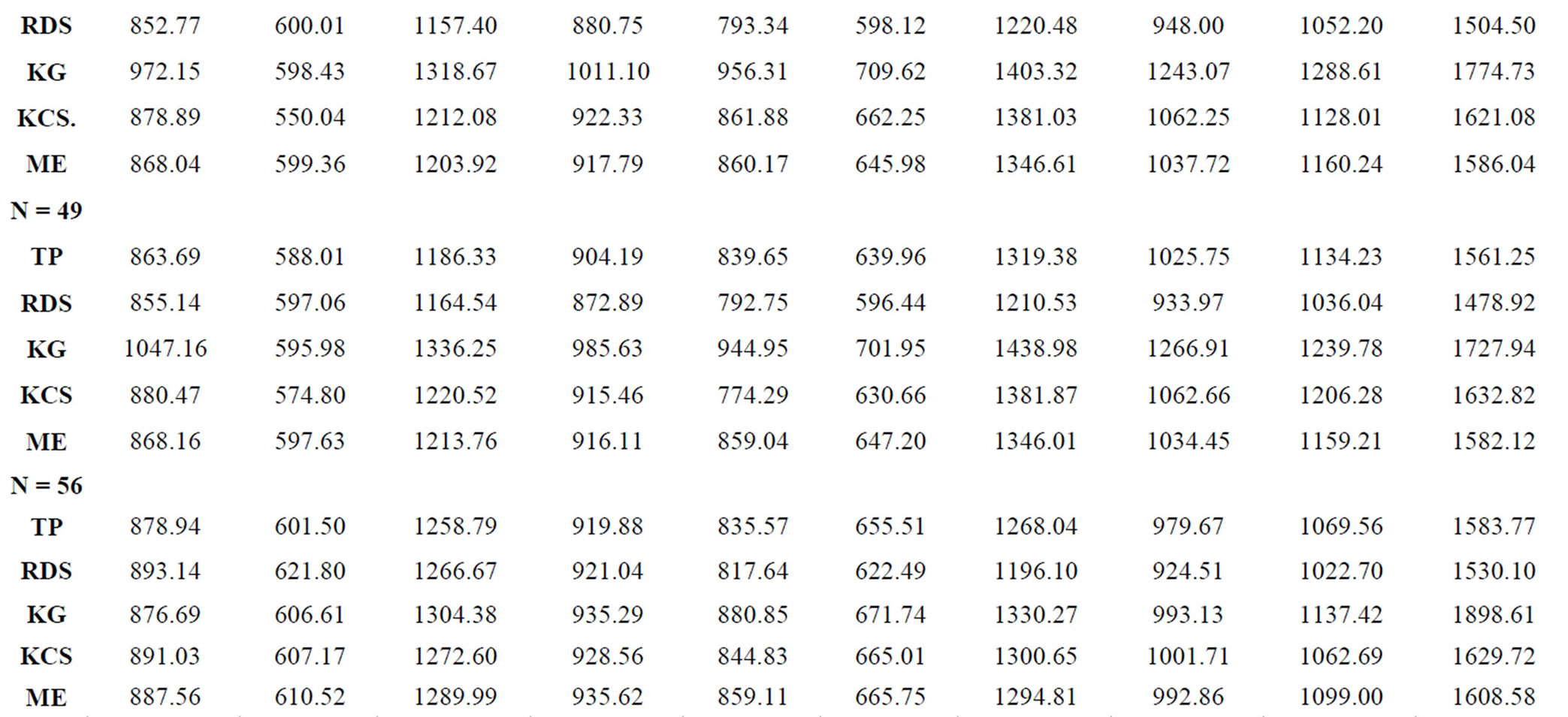
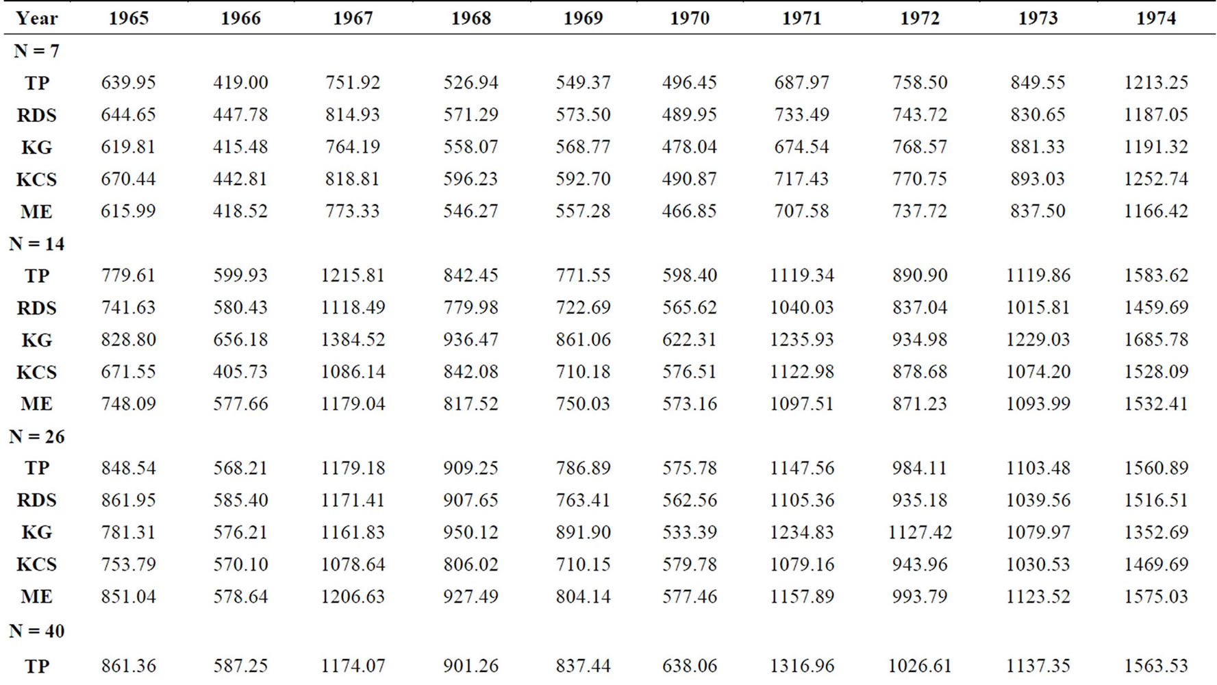
Table 1. Average annual rainfalls (in mm) obtained from each method and scenario.
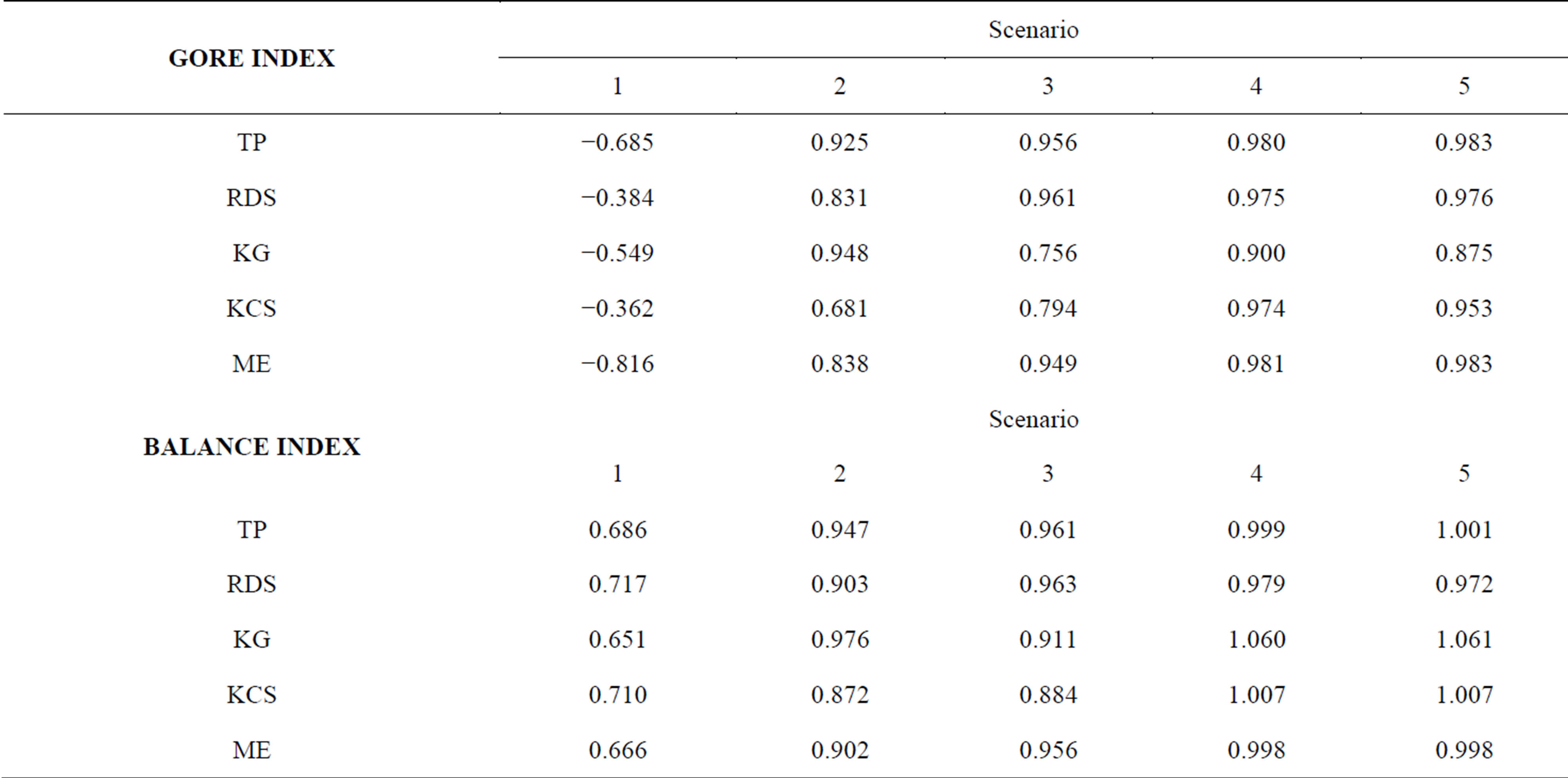
Table 2. GORE and BALANCE results using scenario 6 as reference.
by each method, comparing Scenarios 1 to 5 with the reference 6. From Table 1, is possible to notice that reducing spatial data resulted in a general underestimation of annual mean rainfall. However, all techniques were exposed to the same data conditions and so, it is believed that they can be analyzed directly.
It can observe that all methods, at Scenario 1, gave not so good results, with negative values. In general, indices had a trend of improvement when the number of rain gauges was increased, but it should be noted the irregular behavior presented by both KG and KCS. Despite the KCS having shown the best results in Scenario 1, it just returned to give good results in Scenario 4, but not so good as TP, RDS nor ME. On the other hand, KG showed good results for Scenario 2, but with the worse estimated results for Scenarios 4 and 5, demonstrating a significant instability. Thus, differently of other techniques, the KM was the only method that not presented the improvement behavior in results expected when increasing the data availability. So, results demonstrates that applying of geostatistical techniques on rainfall data needs preliminary studies of data employed and variogram model applied.
It can also verify that TP got an excellent performance from Scenario 2 onwards, for both indices. At this point, it should be noted that care should be taken with this technique. TP ponders the rainfall measures based on the area of influence of each station within the basin, which implies that a good homogeneity combined with an enough density may result reliable values for average rainfall, as seen here. However, in tiny scales of time or bad spatial distribution of data, the rainfall variability, or even the existence of error in the records, can contribute greatly to a discrepant with reality because of method formulation. Moreover, the use of the TP is not suitable for the estimation of rain in a certain region or point in the basin.
ME and RDS also presented great results, very similar, with some emphasis for ME at Scenarios 2, 4 and 5. Both showed the expected behavior improves, as TP did, when increasing the stations numbers. The ME has the advantage, given its theoretical base, that weights estimation, for all stations, are determined simultaneously, which allows possible registry errors may be diluted, resulting in a rainfall surface more reliable than that given by RDS. In other words, ME assesses the spatial structure of the events. As to results, in specific for BALANCE index, RDS obtained better results just at scenarios 1 and 3, pointing out that in the first one all methods were flawed in determining the average rainfall, underestimating its value significantly.
4. Conclusions
The direct comparison among techniques of average rainfall estimation is not possible because the real values are generally unknown. However, this research brought another approach in order to compare indirectly some methods, using not just the results obtained, sometimes very similar, but analyzing the data requiring each one to reach better results given in the best spatial data scenario, in other words, comparing their convergence behavior using GORE and BALANCE indices. The expected behavior from each technique was the continuous improvement in estimated results when increasing spatial data density. Thus, it is reasonable to infer that some methods are appropriate, with a good performance, when their behavior shows that, even with a small amount of data in space, their results approach those that would be given in better conditions.
The results for GORE and BALANCE indices, indicate that TP, RDS and ME as methods are to be applied with satisfaction to obtain the average rainfall value over an area. On the other hand, KM, tested with two variograms models, had a not expected unstable behavior.
Reflecting the need of preliminary studies about data and variograms to be applied, it means a disadvantage given by an increased complexity, especially from the point of view of procedures automation and management tools.
Returning to the methods with a good performance, emphasis must be given to ME, by the great results obtained and its formulation, which helps to mitigate casual data errors allowing estimating a continuous rainfall surface. Still, the study was done in a semi-arid region of Brazil, where pluvial behavior presents a high variability, even in larger time scales, reinforcing the results reached.
It is suggested that more studies be done in this way of indirect comparison of techniques, despite the technological advances, there are many regions where the rainfall monitoring is still scarce and there is a need for reliable water resources planning tools. In the same vein presented here, larger scenarios combinations may be done, using different watersheds and spatial and temporal discretization, so that the methods could be evaluated under various conditions.
Acknowledgements
The authors are deeply grateful to CNPq for Masters Scholarship to Fernando D. Barbalho (Proc. 556625/ 2009-9) and a Productivity Research Grant to Klebber T. M. Formiga (Proc. 310389/2012-7); as well as to the FINEP/CT-HIDRO/PROCESSOS HIDRÁULICOS/2007 to support this research and Federal University of Goiás (UFG) for providing infrastructural conditions for the development of this research.
REFERENCES
- F. Anctil, N. Lauzon, V. Andréassian, L. Oudin and C. Perrin, “Improvement of Rainfall-Runoff Forecasts through Mean Areal Rainfall Optimization,” Journal of Hydrology, Vol. 382, No. 3-4, 2006, pp. 717-725. http://dx.doi.org/10.1016/j.jhydrol.2006.01.016
- H. Wheater, S. Sorooshian and K. D. Sharma, “Hydrological Modelling in Arid and Semi-arid Areas,” Cambridge University Press, New York, 2008.
- C. Cheng, Q. Li, G. Li and H. Auld, “Climate Change and Heavy Rainfall-Related Water Damage Insurance Claims and Losses in Ontario, Canada,” Journal of Water Resource and Protection, Vol. 4, No. 2, 2012, pp. 49-62. http://dx.doi.org/10.4236/jwarp.2012.42007
- V. Andréassian, C. Perrin, C. Michel, I. Usart-Sanchez and J. Lavabre, “Impact of Imperfect Rainfall Knowledge on the Efficiency and the Parameters of Watershed Models,” Journal of Hydrology, Vol. 250, No. 1-4, 2001, pp. 206-223. http://dx.doi.org/10.1016/S0022-1694(01)00437-1
- L. Nicótina, E. A. Celegon, A. Rinaldo and M. Marani, “On the Impact of Rainfall Patterns on the Hydrologic Response,” Water Resources Research, Vol. 44, 2008, pp. 1-14.
- P. M. Younger, J. E. Freer and K. J. Beven, “Detecting the Effects of Spatial Variability of Rainfall on Hydrological Modelling Within an Uncertainty Analysis Framework,” Hydrological Processes, Vol. 23, No. 14, 2009, pp. 1988-2003. http://dx.doi.org/10.1002/hyp.7341
- D. Zoccatelli, M. Borga, F. Zanon, B. Antonescu and G. Stancalie, “Which Rainfall Spatial Information for Flash Flood Response Modelling? A Numerical Investigation Based on Data from the Carpathian Range, Romania,” Journal of Hydrology, Vol. 394, No. 1-2, 2010, pp. 148- 161. http://dx.doi.org/10.1016/j.jhydrol.2010.07.019
- T. Tao, B. Chocat, S. Liu and K. Xin, “Uncertainty Analysis of Interpolation Methods in Rainfall Spatial Distribution—A Case of Small Catchment in Lyon,” Journal of Water Resource and Protection, Vol. 1, No. 2, 2009, pp. 136-144. http://dx.doi.org/10.4236/jwarp.2009.12018
- A. Shaban, C. Robinson and F. El-Baz, “Using MODIS Images and TRMM Data to Correlate Rainfall Peaks and Water Discharges from the Lebanese Coastal Rivers,” Journal of Water Resource and Protection, Vol. 1, No. 4, 2009, pp. 227-236. http://dx.doi.org/10.4236/jwarp.2009.14028
- E. M. Biggs and P. M. Atkinson, “A Comparison of Gauge and Radar Precipitation Data for Simulating an Extreme Hydrological Event in the Severn Uplands, UK,” Hydrological Processes, Vol. 25, No. 5, 2011, pp. 795- 810. http://dx.doi.org/10.1002/hyp.7869
- T. Hu and J. P. Desai, “Soft-Tissue Material Properties under Large Deformation: Strain Rate Effect,” Proceedings of the 26th Annual International Conference of the IEEE EMBS, San Francisco, 1-5 September 2004, pp. 2758-2761.
- Q. Zhou, G. Liu and Z. Zhang, “Improvement and Optimization of Thiessen Polygon Method Boundary Treatment Program,” 17th International Conference on Geoinformatics, 12-14 August 2009, pp. 1-5.
- A. D. Nicks, “Space-Time Quantification of Rainfall Inputs For Hydrological Transport Models,” Journal of Hydrology, Vol. 59, No. 3-4, 1982, pp. 249-260. http://dx.doi.org/10.1016/0022-1694(82)90090-7
- K. N. Dirks, J. E. Hay, C. D. Stow and D. Harris, “HighResolution Studies of Rainfall on Norfolk Island: Part II: Interpolation of Rainfall Data,” Journal of Hydrology, Vol. 208, No. 3-4,1998, pp. 187-193. http://dx.doi.org/10.1016/S0022-1694(98)00155-3
- C. Caruso and F. Quarta, “Interpolation Methods Comparison,” Computers & Mathematics with Applications, Vol. 35, No. 2, 1998, pp. 109-126. http://dx.doi.org/10.1016/S0898-1221(98)00101-1
- C. C. Balascio, “Multiquadric Equations and Optimal Areal Rainfall Estimation,” Journal of Hydrology Engineering, Vol. 6, No. 6, 2001, pp. 498-505. http://dx.doi.org/10.1061/(ASCE)1084-0699(2001)6:6(498)
- G. Matheron, “The Theory of Regionalized Variables and its Applications,” 5. Edition, École national supérieure des mines, Virginia, 1971.
- O. Dubrelet, “Comparing Splines and Kriging,” Computer and Geociences, Vol. 10, No. 2-3, 1984, pp. 327-338. http://dx.doi.org/10.1016/0098-3004(84)90030-X
- V. P. Singh, “Hydrologic Systems—Watershed Modeling Vol. 2,” Prentice Hall, New Jersey, 1988.
- R. L. Hardy, “Multiquadric Equations of Topography and Other Irregular Surfaces,” Journal of Geophysical Research, Vol. 76, No. 8, 1971, pp. 1905-1915. http://dx.doi.org/10.1029/JB076i008p01905
- E. M. Shaw and P. P. Lynn, “A Real Rainfall Evaluation Using Two Surface Fitting Techniques,” Bulletin of the International Association of Hydrological Sciences, Vol. 17, No. 4, 1972, pp. 419-433. http://dx.doi.org/10.1080/02626667209493855
- P. S. Lee, P. P. Lynn and E. M. Shaw, “Comparison of Multiquadric Surfaces for the Estimation of Areal Rainfall,” Hydrological Sciences Journal, Vol. 19, No. 3, 1974, pp. 303-317.
- M. Borga and A. Vizzaccaro, “On the Interpolation of Hydrologic Variables, Formal Equivalence of Multiquadric Surface Fitting and Kriging,” Journal of Hydrology, Vol. 195, No. 1-4, 1997, pp. 160-171. http://dx.doi.org/10.1016/S0022-1694(96)03250-7
- H. K. Syed, D. C. Goodrich, D. E. Myers and S. Sorooshian, “Spatial Characteristics of Thunderstorm Rainfall Fields and Their Reaction to Runoff,” Journal of Hydrology, Vol. 271, 2003, pp. 1-21. http://dx.doi.org/10.1016/S0022-1694(02)00311-6
- S. J. Cole and R. J. Moore, “Hydrological Modelling Using Rain Gauge and Radar-Based Estimators of Areal Rainfall,” Journal of Hydrology, Vol. 358, No. 3-4, 2008, pp. 159-181. http://dx.doi.org/10.1016/j.jhydrol.2008.05.025
- J. C. Ribot, A. R. Magalhães and S. S. Panagides, “Climate Variability, Climate Change and Social Vulnerability in the Semi-arid Tropics,” Cambridge University Press, New York, 2005.
- C. Obled, K. Wendling and K. Beven, “The Sensitivity of Hydrological Models to Spatial Rainfall Patterns: An Evaluation Using Observed Data,” Journal of Hydrology, Vol. 159, No. 1-4, 1994, pp. 305-333. http://dx.doi.org/10.1016/0022-1694(94)90263-1
- A. H. Thiessen, “Precipitation Averages for Large Areas,” Monthly Weather Review, Vol. 39, No. 7, 1911, pp. 1082- 1084. http://dx.doi.org/10.1175/1520-0493(1911)39<1082b:PAFLA>2.0.CO;2
- C. Damant, G. L. Austin, A. Bellon and R. S. Broughton, “Erros in the Thiessen technique for Estimating Areal Rain Amounts Using Weather Radar Data,” Journal of Hydrology, Vol. 62, No. 1-4, 1983, pp. 81-94. http://dx.doi.org/10.1016/0022-1694(83)90095-1
- T. C. Wei and J. L. McGuinness, “Reciprocal Distance Squared Method, a Computer Technique for 309 Estimating Area Precipitation,” Technical Report ARS-Nc-8. US Agricultural Research Service, North 310 Central Region, Ohio, 1973.
- E. C. G. Camargo, S. Drucks and G. Câmara, “Análise Espacial de Superfícies,” In: Análise Espacial de Dados Geográficos, EMBRAPA, Brasília, 2004. (in Portuguese)