Journal of Water Resource and Protection
Vol. 5 No. 3A (2013) , Article ID: 29229 , 13 pages DOI:10.4236/jwarp.2013.53A036
Effect of Freshwater Influx on Phytoplankton in the Mandovi Estuary (Goa, India) during Monsoon Season: Chemotaxonomy
1National Institute of Oceanography, Dona Paula, Goa, India
2Lamont Doherty Earth Observatory at Columbia University, New York, USA
Email: sgpm@nio.org, psushma@nio.org, helga@ldeo.columbia.edu, jig@ldeo.columbia.edu
Received December 22, 2012; revised January 23, 2013; accepted February 2, 2013
Keywords: Phytoplankton; Pigment Analysis; Monsoon; Freshwater Runoff; CHEMTAX
ABSTRACT
The Mandovi estuary is a prominent water body that runs along the west coast of India. It forms an estuarine network with the adjacent Zuari estuary, connected via the Cumbharjua canal. The physico-chemical conditions seen in the Mandovi estuary are influenced by two factors: the fresh water runoff during the monsoon season (June-September) and the tidal influx of coastal seawater during the summer (October to May) season. However, the effects of monsoon related changes on the phytoplankton of the Mandovi estuary are not yet fully understood. An attempt to understand the same has been made here by applying the process of daily sampling at a fixed station throughout the monsoon season. It was noticed that the onset of the monsoon is responsible for an increase in nitrate levels upto 26 μM from <1 µM during pre-monsoon and enhancement of chlorophyll a (chl a) as high as 14 µg·L−1 during the same period. The phytoplankton population was observed through both chemotaxonomy and microscopy and was found to be composed mainly of diatoms. CHEMTAX analysis further uncovers the presence of several other groups of phytoplankton, the presence of which is yet to be reported in many other tropical estuaries. It includes chrysophytes, cyanobacteria, prasinophytes, prymnesiophytes and chlorophytes. The appearance of phytoplankton groups at various stages of the monsoon was recorded, and this data is discussed in relation to environmental changes in the Mandovi estuary during the monsoon season.
1. Introduction
Estuaries are complex ecosystems which have been proven to be interesting areas of study due to their constantly changing physico-chemical environments. Estuaries on the west coast of India are unique in both their physical and biogeochemical features, due to intense freshwater flux during the monsoon [1]. The Mandovi estuary is located between 15˚25'N to 15˚31'N and 73˚45' to 73˚59'E along the west coast of India and is well mixed throughout the year with the exception of the monsoon months during which time vertical stratification appears [2]. The Mandovi estuary receives an annual rainfall of 250 - 300 cm·year−1 during the southwest monsoon (June-September) and less than 10 cm·year−1 during the rest of the year [3]. During the southwest monsoon (SWM), the Mandovi estuary receives heavy freshwater discharge which results in constant alteration in the salinity. Thus the salinity varies from 0 to 22 PSU during the months from June to September [4]. These variations also bring changes in water turbidity and hence availability of solar radiation during the monsoon.
A unique feature of the Mandovi River is the phenomenal tides that it is subject to [5]. As a consequence, the Mandovi estuary experiences large influxes of seawater during the non-monsoon months which not only has a significant impact on its salinity [5,6] but also on its nutrient concentration [7]. Earlier it was noticed that the distribution and abundance of phytoplankton were strongly regulated by both salinity and nutrients [8]. As an alternative and complement to microscopic examination, the accessory pigments estimated by High Performance Liquid-Chromatography (HPLC) provide accurate classspecific differentiation of the phytoplankton groups [9]. This approach has greatly advanced our understanding of phytoplankton pigment composition and functionality in response to ecosystem changes in the southeastern US estuaries [10], the Nervious estuary [11], the Tagus estuary [12] and the Schelde estuary [13], However, this aspect of research is yet to be conducted in Indian estuaries.
The aim of our study was to investigate the response of the phytoplankton community of the Mandovi estuary to monsoonal forcing using HPLC technique and to compare it through microscopy. To the best of our knowledge our study represents the first detailed study of the phytoplankton community combined with a pigments signature in a tropical monsoon-influenced estuary. Our results also provide a further understanding of the dynamics of phytoplankton in neritic environments.
2. Materials and Methods
2.1. Study Site
A 187-day sampling regime was undertaken in the Mandovi estuary (Figure 1). Though partially landlocked, this estuary is exposed to constant flushing and flooding by semidiurnal tides [1]. Water samples were collected daily at 11.0 hrs from the station denoted as A in Figure 1. This site was chosen not only because of its easy access to the coastal research vessel CRV Sagar Shukti, which was anchored at the site during the entire study period, but also on account of the large salinity range (0 to 22 PSU) which the site experiences following the onset of the monsoon season (Shetye et al. 2007). The 187-day study period has been partitioned into four phases based on the rainfall that St. A received during that year: the pre-monsoon (PreM; 23rd May-27th May 2007, Julian Days (JD) 143 - 147), intermonsoon (InterM; 28th May-23rd June 2007, JDs 148 - 174), monsoon (MoN; 24th June to 29th Sep 2007, JDs 175 - 272) and postmonsoon (PostM; 30th Sept-30th Nov JDs 273 - 334) (Pednekar et al., 2011).
Sampling was restricted to the surface and the water was collected using 5 L Niskin sampling bottles, mounted
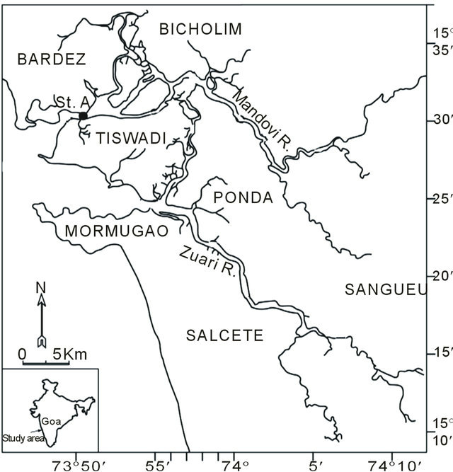
Figure 1. Study area showing sampling station (St. A).
on a Sea Bird Electronics Conductivity Temperature Density (CTD) Rosette. Immediately after collection, the water in the Niskin sampler was carefully drained into acid-washed carboys. Samples were then immediately transported under cold and dark conditions for analysis to the laboratory approximately 10 km away where they were carefully sub-sampled in duplicate for phytoplankton counts by microscopy, HPLC analysis and nitrate analysis. Earlier study revealed the nitrate as important variable whereas other nutrients (phosphate, silicate) do not affect the estuarine ecosystem [14].
2.2. Hydrography
Rainfall data for the Mandovi estuary was obtained from the India Meteorological Department while CTD (sea bird) records were used for temperature-salinity purposes. Salinity was confirmed with a Salinometer (Atago S/ Mill®, Japan, Salinity range 0 - 100 PSU) while the Nitrate was analysed using the method outlined in Strickland and Parsons [15].
2.3. Phytoplankton Identification and Enumeration by Microscopy
Samples for total cell counts of phytoplankton and identification by microscopy were collected in duplicate in 500 ml plastic bottles. Samples were then carefully fixed with a few drops of Lugol’s iodine, preserved with 3% buffered formaldehyde and then stored under dark and cool conditions until the time of analysis [16].
2.4. HPLC Pigment Analysis
The Seawater samples (1 litre) were filtered through GF/F filters and analyzed by HPLC [9,17]. Prior to the HPLC analysis, the filters were immersed in 90% acetone, extracted under cold and dark conditions overnight, sonicated and finally filtered through 0.2 µm, 13 mm PTFE filters to rid the sample of particulate debris. Aliquots of 1 ml of the pigment extract were then mixed with 0.3 ml of distilled water in a 2 ml amber vial and allowed to equilibrate for 5 minutes prior to injection into an HPLC (Agilent® 1100 series) equipped with a diode array detector. Pigments were separated in a C-18 reverse-phase column using the eluent gradient program [9] as adapted by Bidigare and Charles [17] as detailed in Parab, et al. [16]. Chlorophyll, carotenoids and xanthophylls were detected by their absorbance peaks at 436 nm and identified by comparison with the retention times of standard pigments obtained from DHI® Water and Environment, Denmark. The following abbreviations are used for the pigments: chlorophyll a (chl a), chlorophyll c2 (chl c2), fucoxanthin (fuco), diadinoxanthin (diad), peridinin (peri), zeaxanthin (zea), alloxanthin (allo), prasinoxanthin (pras), 19’hexanoyloxyfucoxanthin (19’hex), 19’butanoyloxyfucoxanthin (19’but), lutein (lut), neoxanthin (neo) and myxoxanthophyll (myxo).
2.5. Chemotaxonomic Analyses of Phytoplankton
The Algal class abundance was determined from HPLC algal pigment measurements using CHEMTAX, a factor analysis programme, which estimates the contribution of each specified phytoplankton pigment class to the total chl a concentration in a water sample [18].
2.6. Statistical Analysis
The Principal component analysis (PCA) was carried out using Statistical package version 6.0. (Statsoft, Oklahoma USA). The first principal component Factor 1 accounts for greater variability and each succeeding factor explains the remaining variability possible in the data set. The ordination results for the first two most important factors (Factor 1 and Factor 2) were retained. The average tide for one week cycle is compared with biological data to normalize daily tide variability at a fixed time.
3. Results
3.1. Physico-Chemical Conditions of the Estuary
During PreM season (JD 143) corresponding with the first rain showers the salinity was 37 ± 2. The intense rain received during JDs 148 - 272 brought about drastic changes in the salinity of the region under study. Initially salinity was slowly lowered from 0 - 20 during JDs 175 - 272. At the end of the MoN salinity showed upwards trend and the PostM season (JDs 273 - 334) was marked by the presence of moderate salinity at the study site (26 ± 7). These variations in salinity occurring with rainfall are depicted in Figure 2, where salinity followed the pattern of the rain received.
Land runoff during the MoN brought nitrate into the estuary, thus increasing its concentration up to 26 µM. The progression of the monsoon witnessed the addition and dilution of nitrate due to the freshwater runoff this in turn was also responsible for the moderately high nitrate levels (in the range of 10 - 15 µM) throughout the monsoon (Figure 3).
The salinity and temperature data recorded by CTD during daily sampling is compiled. Temperature was not important factor since this is a shallow part of estuary near to river mouth. However stratification was due to the freshwater cap formed during active monsoon. During the PreM, the temperature of the water column was around 31˚C while its salinity was around 36. As the monsoon progressed the temperature was lowered to 26˚C and salinity nearly zero with stratified water column. The PostM season was marked by 29˚C water temr
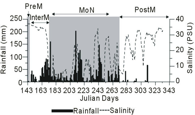
Figure 2. Variation in salinity and RAINFALL in Mandovi estuary. Where 143 - 147 (PreM), 148 - 174 (InterM), 175 - 272 (MoN) and 273 - 334 (PostM).
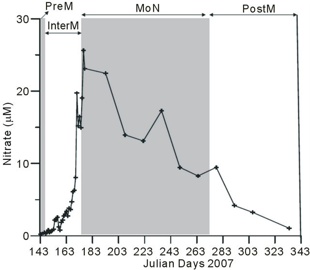
Figure 3. Variation in nitrate in Mandovi estuary. Where 143 - 147 (PreM), 148 - 174 (InterM), 175 - 272 (MoN) and 273 - 334 (PostM).
perature and around 20 salinity with well mixed water column (Figure 4).
3.2. Microscopic Study
Phytoplankton cell numbers were found to be highest at the beginning of the monsoon, in the range of (2 - 6.5) × 104 cells·L−1. During the InterM period high counts of the filamentous cyanobacteria Trichodesmium erythraeum and Trichodesmium thiebautii ranging from 0.001 - 1.286 × 10⁴ filaments·L−1 were recorded in the Mandovi estuary. During the MoN the population of the phytoplankton increased time to time due to a break in the monsoonal rainfall (Figure 5). An increase of at least six fold was recorded in phytoplankton numbers during the MoN while a three fold increase was recorded during the PostM compared to low values during intense monsoon (Figure 5). Monsoon pattern of total phytoplankton counts was more similar to diatom counts where as
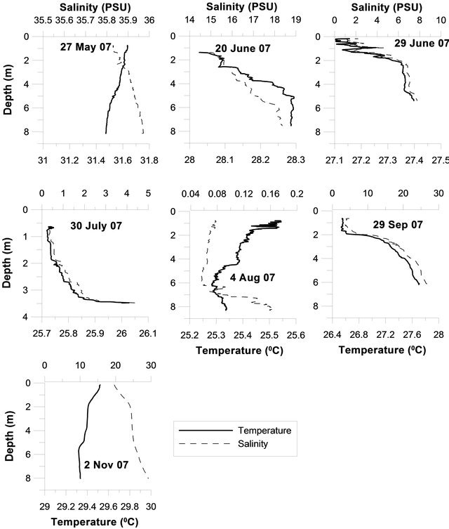
Figure 4. Temperature and salinity variations in the Mandovi estuary.
PostM matched with dinoflagellates counts (JDs 285, 303 and 350). This increase during MoN was associated with blooms of the diatom Skeletonema costatum where its cells varied from (2 - 6)× 104 cells·L−1. In case of the PostM, the counts of the dinoflagellate Scrippsiella trochoidea were found to be in the range of (1 - 3)× 104 cells·L−1 altering the phytoplankton pattern (Figure 5).
3.3. Phytoplankton Pigments and CHEMTAX Study
Chlorophyll a which is the indicator of phytoplankton biomass is higher during InterM (5.76 ± 1 µg·L−1) compared to other seasons which varied from 1.95 - 2.96 µg·L−1. Similarly, chl b, chl c2, fuco and peri were also high during InterM period (Table 1). Other pigments like pras, allo, lut, myxo, 19’ but and 19’ hex were low during entire study period. Group level information on phytoplankton derived from chemtax study using pigment estimates is presented as the chl a equivalent to a particular phytoplankton group. At the beginning of the monsoon the increase in the chl a was mainly due to diatom growth (Figure 6), followed by cryptophytes. At the end of the MoN, an increase in the dinoflagellate population was recorded. Three prominent peaks of the prymnesiophytes were recorded during a break in the MoN where salinity was on the rise. The PostM season was also marked by an increase in the population of picocyanobacteria and prasinophytes during intermittent showers of the post-monsoon rain. It was also observed that all six groups of phytoplankton recorded by CHEMTAX study appeared as mixed populations just after the first showers of the MoN during JDs 148 - 174 where salinity and nitrate both were high.
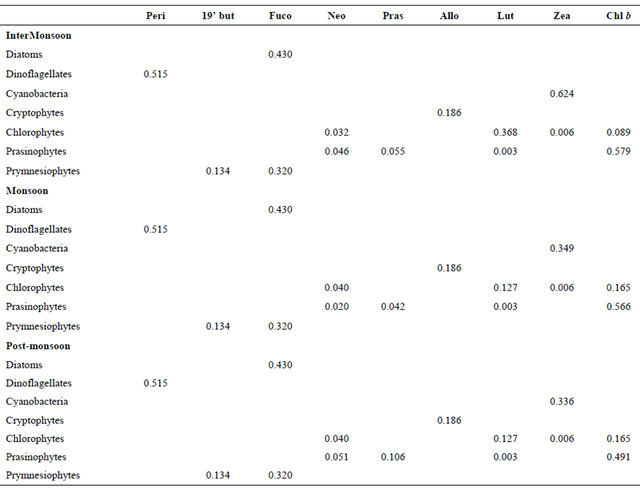
The final output ratio matrices for InterM, MoN and PostM are shown in Table 2. The relative contribution of pigment groups to Chl a is illustrated in Table 3. The mean percentage of diatoms by CHEMTAX was high during InterM (63%) and PostM (63%) and low in the PreM (42 %; Table 3). Dinoflagellates were high in the PostM (10%), cryptophytes in the MoN (22%), prymnesiophytes in the InterM (1%) whereas cyanobacteria and prasinophytes during PreM (40% and 6% respectively; Table 3).
3.4. Comparison of Microscopy and CHEMTAX Study
Out of the six groups of phytoplankton recorded by
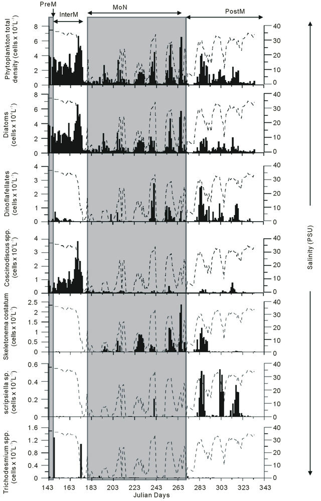

Figure 5. Biomass chlorophyll a, total phytoplankton density and dominant species in the Mandovi estuary during monsoon.
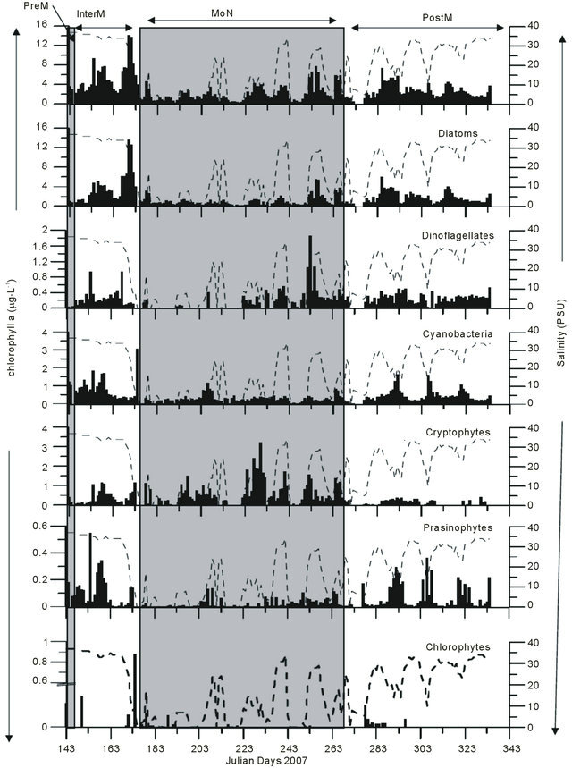

Figure 6. Phytoplankton groups revealed by CHEMTAX and Salinity variation.
Table 1. Phytoplankton average pigments and salinity during monsoon study in the Mandovi estuary.
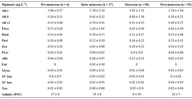
NC indicates samples not collected.
Table 2. Output ratios for each season as calculated by CHEMTAX.
CHEMTAX study, only the diatoms and the dinoflagellates were examined by the microscopy (Figure 5). Further it was noticed that the diatom being major group was in agreement with the CHEMTAX derived diatom data (Figure 6). This was also observed during bloom of the Skeletonema costatum, during intermittent break in the rain and increase in the salinity.
3.5. Effect of Environmental Variables on the Phytoplankton Population
To know whether the variations in the hydrography, and phytoplankton biomass by microscopy and HPLC due to the tidal advection, the running 14 days mean was taken (Figure 7). It was found that the salinity varied from 2.86 - 36 (ave. 15 ± 11), chl a varied from 1.23 - 6.41
Table 3. Mean (plus the standard deviations) contribution of phytoplankton classes to chlorophyll a biomass (expressed in percentage) calculated by CHEMTAX.
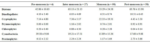
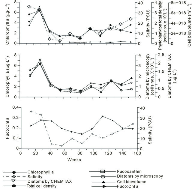
Figure 7. Pigment:chl a ratio and salinity in Mandovi estuary during the Monsoon season.
µg·L−1 (ave. 2.86 ± 1.48), total phytoplankton density ranged from 0.52 - 3.21 cell nos. × 104 L−1 (1.42 ± 0.88), cell biovolume was 2e+017 - 7e+018 m3·L−1 (1e+018 ± 2e+018), fuco was 0.18 - 1.74 µg·L−1 (0.63 ± 0.43), diatoms by microscopy ranged from 0.49 - 3.13 cell nos. × 104 L−1 (1.20 ± 0.88), diatoms by CHEMTAX was 0.24 - 2.21 µg·L−1 (0.79 ± 0.56) and fuco:chl a ratio was 0.14 - 0.31 (0.22 ± 0.05).
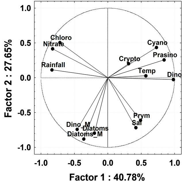
To discriminate patterns of variation in the phytoplankton groups by CHEMTAX during different seasons, PCA analysis was undertaken using all phytoplankton groups derived by CHEMTAX and environmental variables (salinity, temperature, rainfall and nitrate) as input variables. During InterM the first two factors, Factors 1 and 2, explained 34.66% and 17.84%; MoN, 45.71% and 19.26% and PostM 40.78% and 27.65% respectively, of the total variation in the phytoplankton groups by CHEMTAX (Figure 8(a)). During InterM, diatoms by CHEMTAX as well as microscopy showed a positive correlation with rainfall and nitrate, while temperature was negatively correlated with these groups (Figure 8(a)). Rainfall and nitrate were negatively correlated with all phytoplankton groups during MoN while salinity was positively correlated with diatoms, cryptophytes and cyanobacteria (Figure 8(b)). In PostM, rainfall and nitrate were negatively correlated with most of the phytoplankton groups except for chlorophytes (Figure 8(c)).
4. Discussion
Marine ecosystems are sensitive to physical factors like stratification, solar input and temperature and chemical factors like nutrients, salinity and oxygen content of the water mass. In an estuarine ecosystem, in addition to these factors, freshwater runs off during the MoN also to be taken into consideration. The land runoff during the monsoon transports fertilizers and organic detritus from surrounding agricultural areas, which in turn alter the light penetration due to an increase in the turbidity and resuspension of the bottom sediment [7]. During 2007, the monsoon was well spread and the salinity changes in the Mandovi estuary matched the rainfall pattern (Figure 2). It is interesting to note that, during the monsoon study for 10 - 12 times salinity reached to 0 PSU indicating that a total flushing of the estuarine water was taking place, thereby making the estuary a freshwater system. From temperature and salinity data (Figure 4) it appears that Mandovi estuary was stratified during the entire MoN whereas well mixed during PreM and PostM season. Mandovi estuary have identified as partial-stratified estuary [1].
During the peak of the MoN nitrate was as high as 26 µM and remained more than 5 µM throughout the monsoon (Figure 3). Our nitrate value was higher than the earlier reports from Mandovi estuary which was 6 - 11 µM [20,21]. The increase in nitrate in the estuary over the years is appreciable, that may be due to agricultural runoff during the monsoons and process of eutrophication due to industrialization of catchment area and overuse of river water for ore transport, drinking and agriculture usage.
 (a)
(a)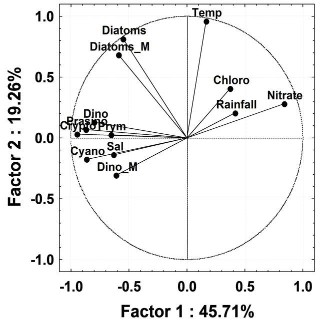 (b)
(b)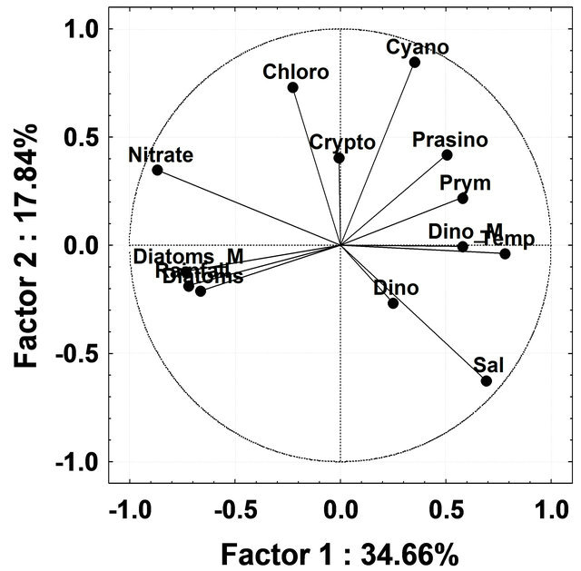 (c)
(c)
Figure 8. (a) Principal Component Analysis ordination diagram relative to data on absolute contribution of phytoplankton groups by CHEMTAX and microscopy and physicochemical parameter during Intermonsoon in the Mandovi estuary. Symbols represents Dino-dinoflagellates; Cyano-cyanobacteria; Crypto-cryptophytes; Chloro-chlorophytes; Prymprymnesiophytes; Prasino-prasinophytes; Diatom_M-diatoms by microscopy; Dino_M-dinoflagellates by microscopy; Temp-temperature and Sal-salinity; (b) Principal Component Analysis ordination diagram relative to data on absolute contribution of phytoplankton groups by CHEMTAX and microscopy and physicochemical parameter during Monsoon in Mandovi estuary. Symbols are represented with the same used in Figure 8(a); (c) Figure 8(c) Principal Component Analysis ordination diagram relative to data on absolute contribution of phytoplankton groups by CHEMTAX and microscopy and physicochemical parameter during post-monsoon in the Mandovi estuary. Symbols are represented with the same used in Figure 8(a).
The impact of the monsoon on the phytoplankton population was recorded in terms of the phytoplankton (total cell numbers and chlorophyll a) and percentage of the phytoplankton groups [19]. The phytoplankton counts during the MoN were 3.63 ± 0.86 nos. × 104 L−1 which was higher than the PostM (0.98 ± 0.962 nos. × 104 L−1) and close to the PreM (3.42 ± 0.66 nos. × 104 L−1) period. The earlier reports on phytoplankton counts and chl a concentration of Mandovi estuary during the MoN was much lower [22] as compared to the rest of the year. Our data shows that the phytoplankton biomass is negatively affected during monsoon and not severely affected as it was reported earlier [22]. On the contrary, the diversity of phytoplankton was more during monsoon compared to other seasons [19].
In the backwaters of Cochin (India), with a similar estuarine system along the west coast of India, the phytoplankton biomass was found to be greater during the peak monsoon season [23]. However, blooms of Ceratium furca and Nitzschia closterium was observed during the PostM in the Mandovi estuary [22]. The fact that during the PostM dinoflagellate population is more important part of the succession of the phytoplankton recorded in the Mandovi estuary [19].
The chlorophyll a distribution pattern during the monsoon season in the estuary matches with the salinity pattern and hence rain. These peaks were composed of blooms of diatoms (monsoon) and dinoflagellates (postmonsoon). Further it was noticed that Skeletonema costatum was the most successful diatom species during the monsoon while the dinoflagellate Scrippsiella trochoidea was during MoN and PostM (Figure 5). During monsoon stratification has supported diatom growth as long as nitrate level was high. At the end of the monsoon stratification persist but low nitrate only supported dinoflagellates. The large amount of biomass produced by Skeletonema costatum is exported to nearby coastal waters where it is recycled further, enrichment source of coastal waters during monsoon [16]. The west coast of Goa is rich in fishery [24] and this river plays an important role by export of organic matter during MoN and PostM seasons.
The phytoplankton counts data was in agreement with chl a (Figure 7). The relationship between chl a and total phytoplankton by microscopy is significant (r2 = 0.6; n = 187), where microplankton is the important size group of the phytoplankton in the Mandovi estuary. The effect of the monsoon runoff on both diatom and dinoflagellate populations has been recently published (Pednekar et al., 2011). We have used this data with pigment data in Figure 5 the indicative pigments like fucoxanthin (for diatom) and peridinin (for dinoflagellates) reflects on taxonomic data. Thus, pigment signatures are reliable tool for understanding impact of environmental changes on phytoplankton population in the tropical estuaries like Mandovi estuary.
Although cryptophytes, chlorophytes, prasinophytes and cyanobacteria are important components of the Mandovi estuary the pattern of the phytoplankton community can be understood by study of the diatom and the dinoflagellate population (Figure 6). The fuco:chl a ratio remained same throughout the monsoon season (0.43). Similar data is also reported in the temperate estuarine region [25]. As such fucoxanthin showed a strong correlation with chl a during the study (r2 = 0.8; n = 187). The ratio chl b:chl a during our study varied from 0.089 to 0.579 (Table 2). The highest value was found during the InterM. The chl b has been reported in the small size-phytoplankton in the estuarine waters [11,26]. A high concentration of chl b in the eastern English channel in winter although no green algae were detected by light microscopy suggesting these algae were in picoplankton fraction [27]. In the Nervion river estuary the authors [28] reported Micromonas pusilla as dominant picoplankton. Prasinophytes have also been found to be the dominant green algae in other estuarine areas [29-31]. The ratio of chl b:chl a is higher in prasinophytes than in chlorophytes [32], reaching values upto 0.8 in Micromonas pusilla [33]. The chl b:chl a ratio in the Mandovi estuary was partly due to the prasinophytes in addition to the chlorophytes. The peri:chl a ratio (0.515) for dinoflagellates remained unchanged in the Mandovi estuary which is similar to reported [26,34]. Similarly cryptophytes were a major component of the phytoplankton in the Mandovi estuary also observed in other estuarine and coastal waters [29,35,36]. The allo:chl a ratio (0.186) was similar to the other estuaries reported [37] (0.229); [38] (0.234); [39] (0.278), [40] (0.186), but lower than the earliar reports [11,29]. The zea:chl a ratio for cyanobacteria in the Mandovi estuary was 0.349 during MoN. This value was lower than the reported values for other estuaries [26] (0.846); [29] (1.12); [34] (0.836)]; [41] (1.24); [42] (1.20) and [43] (0.7).
Besides diatoms, a reduction in the number of prasinophytes was also recorded during the MoN period (Figure 6). The occurrence of chlorophytes, cryptophytes and cyanobacteria as important groups of phytoplankton was recorded for the first time from this or any other tropical estuary. High concentrations of the chlorophytes and cryptophytes have been known to prevail in the Kirka River [44], the Hudson River [45], the Urdaibai estuary [37] and the Nervious River [11]. The CHEMTAX analysis employed in our study gives a new insight into the community structure of the phytoplankton in the Mandovi estuary. The CHEMTAX analysis of the Mandovi estuary (Table 3) revealed a decrease in diatoms upto 53% of total phytoplankton and an increase in dinoflagellates upto 11% during PostM (Table 3). Another interesting aspect was that of cryptophytes that increased from 7% to 22% of the phytoplankton population during PreM and MoN. The high percentage of cyanobacteria during the PreM was due to the Trichodesmium erythraeum presence in the Mandovi estuary. The percentage of picocyanobacteria was around 15% - 20% throughout the study, which is reasonably high (Table 3). During the InterM, the increase seen in the diatom population was due to high nitrate levels which was as high as 26 µg·L−1 (Figure 8(a)). However, although nitrate was high, low salinity and low temperature during the monsoon has affected diatom at population level (Figure 8(b)). As the salinity lowered during the monsoon, there was an increase in the prymnesiophytes, prasinophytes, cyanobacteria and cryptophytes. Salinity was showing upward values during PostM and favored diatoms initially and dinoflagellates (Figure 8(c)).
5. Conclusions
Diatoms are an important group of phytoplankton found during the pre-monsoon season. Further, more they are affected by the freshwater that is experienced more during the peak monsoon season. Dinoflagellate bloom of Scrippsiella trochoidea followed bloom of Skeletonema costatum at the end of MoN and continued during PostM season. Besides this, chlorophytes and cryptophytes constitute an important part of the phytoplankton community during monsoon. The presence of the Trichodesmium erythraeum and Trichodesmium thiebautii during PreM and InterM season and pico-cyanobacteria during MoN comprised of as high as 19% of the total phytoplankton biomass. Land runoff was the cause of bloom of the Gyrodinium spirale at the end of the monsoon. Probability of such HAB events in this and the other tropical estuaries suggests the requirement of the phytoplankton monitoring programme in this estuary.
Since samples were collected at fixed time, area is subjected to tidal variation on daily basis. The weekly tidal cycle is characteristics feature. The chl a, phytoplankton numbers, phytoplankton volume, diatom numbers and fuco:chl a ratio are averaged for weekly basis (Figure 7). Effect of monsoon is clearly seen on phytoplankton biomass specially diatom as the group during this averaging exercise (Figure 7). A linear relationship was also existed in chl a to fuco relationship where r2 = 0.8 (n = 187) indicates the importance of diatom in the estuarine region. Such diatom estimated by CHEMTAX and microscopy showed 1:1 relationship on overall basis (r2 = 0.8, n = 187).
6. Acknowledgements We are grateful to Dr. S. R. Shetye, Director, National Institute of Oceanography, Goa for involving us and guiding during the Monsoon Experiment in the Mandovi Estuary. A DST Fellowship to S. G. Parab is gratefully acknowledged. Thanks to Mrs. Suraksha Pednekar and Mr. Subhojit Basu for help during field work. This is an NIO contribution (No. 5319).
REFERENCES
- S. R. Shetye, I. Suresh and D. Sundar, “Tides and Sea Level Variability,” In: S. R. Shetye, D. Kumar and D. Shankar, Eds., The Mandovi and Zuari Estuaries, National Institute of Oceanography, Dona-Paula, 2007, pp. 59.
- K. K. Varma, L. V. G. Rao and C. Thomas, “Temporal and Spatial Variations in Hygrographic Conditions of Mandovi Estuary,” Indian Journal of Marine Science, Vol. 4, 1975, pp. 11-17.
- S. R. Shetye and C. S. Murthy, “Seasonal Variation of Salinity in the Zuari Estuary Goa India,” Proceedings Indian Academic Science (Earth Planet Science), Vol. 96, 1987, pp. 249-257.
- S. R. Shetye, A. D. Gouveia, S. Y. S. Singbal, C. G. Naik, D. Sundar, G. S. and G. M. Nampoothiri, “Propagation of Tides in the Mandovi-Zuari Estuarine Network,” Proceedings Indian Academic Science (Earth Planet Science), Vol. 104, No. 4, 1996, pp. 667-682.
- S. R. Shetye, D. Shankar, N. Singh, N. Suprit, G. S. Michael and P. Chandramohan, “The Environment That Conditions the Mandovi and Zuari Estuaries,” In: S. R. Shetye, D. Kumar and D. Shankar, Eds., The Mandovi and Zuari Estuaries, National Institute of Oceanography, Dona-Paula, 2007, p. 3.
- V. Vijith, D. Sundar and S. R. Shetye, “Time-Dependence of Salinity in Monsoonal Estuaries,” Estuarine, Coastal and Shelf Science, Vol. 85, No. 4, 2009, pp. 601- 608. doi:10.1016/j.ecss.2009.10.003
- S. N. DeSousa, R. SenGupta, S. Sanzgiri and M. D. Rajagopal, “Studies on Nutrients of Mandovi and Zuari River Systems,” Indian Journal of Marine Science, Vol. 10, 1981, pp. 314-321.
- V. P. Devassy and J. I. Goes, “Seasonal Pattern of Phytoplankton Biomass and Productivity in a Tropical Estuarine Complex (West Coast of India),” Proceedings Indian Academic Science (Earth Planet Science), Vol. 99, 1989, pp. 485-501.
- S. W. Wright, S. M. Jeffrey, R. F. C. Mantoura, C. A. Llewellyn, T. Bjornland, D. Repeta and N. Welschmeyer, “Improved HPLC Method for the Analysis of Chlorophylls and Carotenoids from Marine Phytoplankton,” Marine Ecology Progress Series, Vol. 77, 1991, pp. 183- 196. doi:10.3354/meps077183
- A. L. Lewitus, D. L. White, R. G. Tymowki, M. E. Geesey, S. N. Hymel and P. A. Noble, “Adapting the CHEMTAX Method for Assessing Phytoplankton Taxonomic Composition in Southeastern US Estuaries,” Estuaries, Vol. 28, No. 1, 2005, pp. 160-172. doi:10.1007/BF02732761
- S. Seoane, A. Laza and E. Orive, “Monitoring Phytoplankton Assemblages in Estuarine Waters: The Application of Pigment Analysis and Microcopy to Size-Fractionated Samples,” Estuarine and Coastal Shelf Science, Vol. 67, No. 3, 2006, pp. 343-354. doi:10.1016/j.ecss.2005.10.020
- C. Gameiro, P. Cartaxana and V. Brotas, “Environmental Drivers of Phytoplankton Distribution and Composition in Tagus Estuary Portugal,” Estuarine and Coastal Shelf Science, Vol. 75, No. 1-2, 2007, pp. 21-34. doi:10.1016/j.ecss.2007.05.014
- M. Lionard, K. Muylaert, M. Tackx and W. Vyverman, “Evaluation of the Performance of HPLC-CHEMTAX Analysis for Determining Phytoplankton Biomass and Composition in a Turbid Estuary (Schelde, Belgium),” Estuarine and Coastal Shelf Science, Vol. 76, No. 4, 2008, pp. 809-817. doi:10.1016/j.ecss.2007.08.003
- M. V. Maya, R. Agnihotri, A. K. Pratihary, S. Karapurkar, H. Naik and S. W. A. Naqvi, “Variations in Some Environmental Characteristics Including C and N Stable Isotopic Composition of Suspended Organic Matter in the Mandovi Estuary,” Environmental Monitoring, Vol. 175, No. 1-4, 2011, pp. 501-517. doi:10.1007/s10661-010-1547-8
- D. H. Strickland and I. R. Parsons, “A Manual of Seawater Analysis,” Bulletin Fishery Research, Vol. 125, 1965, pp. 65-72.
- S. G. Parab, S. G. Prabhu Matondkar, H. do R. Gomes and J. I. Goes, “Monsoon Driven Changes in Phytoplankton Population in the Eastern Arabian Sea as Revealed by Microscopy and HPLC Pigment Analysis,” Continental Shelf Research, Vol. 26, No. 20, 2006, pp. 2538-2558. doi:10.1016/j.csr.2006.08.004
- R. G. Bidigare and C. T. Charles, “HPLC Phytoplankton Pigments: Sampling Laboratory Methods and Quality Assurance Procedures,” In: G. S. Fargion and J. L. Muellier, Eds., Protocols for Satellite Ocean Colour Validation Revisions, NASA, Greenbelt, 2002, pp. 154-160.
- M. D. Mackey, D. J. Mackey, H. W. Higgins and S. W. Wright, “CHEMTAX—A Programme for Estimating Class Abundance from Chemical Markers: Application to HPLC Measurements of Phytoplankton,” Marine Ecology Progress Series, Vol. 144, 1996, pp. 265-283. doi:10.3354/meps144265
- S. M. Pednekar, S. G. Prabhu Matondkar, H. R. Gomes, J. I. Goes, S. G. Parab and V. Kerkar, “Fine-Scale Responses of Phytoplankton to Freshwater Influx in a Tropical Monsoonal Estuary Following the Onset of Southwest Monsoon,” Journal of Earth System Science, Vol. 120, No. 3, 2011, pp. 545-556. doi:10.1007/s12040-011-0073-6
- S. Z. Qasim and R. SenGupta, “Environmental Characteristics of the Mandovi-Zuari Estuarine System in Goa,” Estuarine Coastal and Shelf Science, Vol. 13, No. 5, 1981, pp. 557-578. doi:10.1016/S0302-3524(81)80058-8
- S. N. De Sousa, “Studies on the Behavior of Nutrients in the Mandovi Estuary during Premonsoon,” Estuarine Coastal and Shelf Science, Vol. 16, No. 3, 1983, pp. 299- 308. doi:10.1016/0272-7714(83)90147-6
- V. P. Devassy and J. I. Goes, “Phytoplankton Community Structure and Succession in Tropical Estuarine Complex,” Estuarine Coastal and Shelf Science, Vol. 27, No. 6, 1988, pp. 671-685. doi:10.1016/0272-7714(88)90074-1
- C. P. Gopinathan, “Seasonal Abundance of Phytoplankton in the Cochin Backwaters,” Journal of Marine Biological Association of India, Vol. 14, 1974, pp. 568-577.
- B. Fernandes and C. T. Achutankutty, “Seasonal Variation in Fishery Diversity of Some Wetlands of the Salcete Taluka Goa,” Indian Journal of Marine Science, Vol. 39, 2010, pp. 238-247.
- S. W. Gibb, D. G. Cummings, X. Irigoien, R. G. Barlow and R. F. C. Mantoura, “Phytoplankton Pigment Chemotaxonomy of the Northeastern Atlantic,” Deep-Sea Research Part II, Vol. 48, 2001, pp. 795-823.
- F. Rodriguez, Y. Pazos, J. Maneiro and M. Zapata, “Temporal Variation in Phytoplankton Assemblages and Pigment Composition at a Fixed Station of the Ria of Pontevedra (NW Spain),” Estuarine and Coastal Shelf Science, Vol. 58, No. 3, 2003, pp. 499-515. doi:10.1016/S0272-7714(03)00130-6
- E. Breten, C. Brunet, B. Sautour and J. M. Brylinski, “Annual Variations of Phytoplankton Biomass in the Eastern English Channel: Comparison by Pigment Signatures and Microscopic Counts,” Journal of Plankton Research, Vol. 22, No. 8, 2000, pp. 1423-1440. doi:10.1093/plankt/22.8.1423
- F. Not, M. Latasa, D. Marie, T. Cariou, D. Vailot and N. Simon, “A Single Species, Micromonas pusilla (Prasinophyceae), Dominates the Eukaryotic Picoplankton in the Western English Channel,” Applied Environmental Microbiology, Vol. 70, No. 7, 2004, pp. 4064-4072. doi:10.1128/AEM.70.7.4064-4072.2004
- J. I. Carreto, N. G. Montoya, H. R. Benavides, R. Guerrero and M. O. Carignan, “Characterization of Spring Phytoplankton Communities in the Rio de La Plata Maritime Front Using Pigment Signatures and Cell Microscopy,” Marine Biology, Vol. 143, No. 5, 2003, pp. 1013- 1027. doi:10.1007/s00227-003-1147-z
- S. E. Lohrenz, C. L. Carroll, A. D. Weidemann and M. Tuel, “Variations in Phytoplankton Pigments Size Structure and Community Composition Related to Wind Forcing and Water Mass Properties on the North Carolina Inter Shelf,” Continental Shelf Research, Vol. 23, No. 14- 15, 2003, pp. 1447-1464. doi:10.1016/S0278-4343(03)00131-6
- L. Schluter and F. Mohlenberg, “Detecting of Phytoplankton Groups with Non-Specific Pigment Signatures,” Journal of Applied Science, Vol. 15, 2003, pp. 465-476.
- P, Henriksen, B. Riemann, H. Kaas, H. M. Sorensen and H. L. Sorensen, “Effect of Nutrient-Limitation and Irradiance on Marine Phytoplankton Pigments,” Journal of Plankton Research, Vol. 24, No. 9, 2002, pp. 835-858. doi:10.1093/plankt/24.9.835
- M. Latasa, R. Scharek, F. Le Gall and L. Guillou, “Pigment Suites and Taxonomic Groups in Prasinophyceae,” Journal of Phycology, Vol. 40, No. 6, 2004, pp. 1149- 1155. doi:10.1111/j.1529-8817.2004.03136.x
- L. A. Martinez, S. Seone, M. Zapata and E. Orive, “Phytoplankton Pigment Patterns in a Temperate Estuary: from Unialgal Cultures to Natural Assemblages,” Journal of Plankton Research, Vol. 29, No. 11, 2007, pp. 913-929. doi:10.1093/plankt/fbm069
- C. Brunet and F. Lizon, “Tidal and Diel Periodicities of Size-Fractionated Phytoplankton Pigment Signatures at an Offshore Station in the Southeastern English Channel,” Estuarine Coastal and Shelf Science, Vol. 56, No. 3-4, 2003, pp. 833-843. doi:10.1016/S0272-7714(02)00323-2
- I. A. Garibotti, M. Vernet, W. A. Kozlowski and M. E. Ferrario, “Composition and Biomass of Phytoplankton Assemblages in Coastal Antarctic Waters: A Comparison of Chemotaxonomic and Microscopic Analyses,” Marine Ecology Progress Series, Vol. 247, 2003, pp. 27-42. doi:10.3354/meps247027
- A. Ansotegui, J. M. Trigueros and E. Orive, “The Use of Pigment Signatures to Assess Phytoplankton Assemblage Structure in Estuarine Waters,” Estuarine Coastal and Shelf Science, Vol. 52, No. 6, 2001, pp. 689-703. doi:10.1006/ecss.2001.0785
- W. W. C. Gieskes and G. W. Kraay, “Dominance of Cryptophyceae during the Phytoplankton Spring Bloom in the Central North Sea Detected by HPLC Analysis and Pigments,” Marine Biology, Vol. 75, No. 2-3, 1983. pp. 179-185. doi:10.1007/BF00406000
- R. G. Barlow, R. F. C. Mantoura, R. D. Peinert, A. E. J. Miller and T. W. Fileman, “Distribution Sedimentation and Fate of Pigment Biomarkers Following Thermal Stratification in the Western Alboran Sea,” Marine Ecology Progress Series, Vol. 125, 1995, pp. 279-291. doi:10.3354/meps125279
- S. W. Wright, D. P. Thomas, H. J. Marchant, H. W. Higgins, M. D. Mackey and D. J. Mackey, “Analysis of Phytoplankton of the Australian Sector of the Southern Ocean: Comparison of Microscopy and Size Frequency Data with Interpretations of Pigment HPLC Data Using the ‘CHEMTAX’ Matrix Factorization Program,” Marine Ecology Progress Series, Vol. 144, 1996, pp. 285-298. doi:10.3354/meps144285
- L. Schluter, F. Mohlenberg, H. Havskum and S. Larsen, “The Use of Phytoplankton Pigment/Chlorophyll a Ratios,” Marine Ecology Progress Series, Vol. 192, 2000, pp. 49-63.
- T. M. Kana, P. M. Gilbert, R. Goericke and N. A. Welschmeyer, “Zeaxanthin and ‘Beta’-Carotene in Synechococcus WH7803 Respond Differently to Irradiance,” Limnology and Oceanography, Vol. 33, No. 6, 1988, pp. 1623-1627. doi:10.4319/lo.1988.33.6_part_2.1623
- A. Morel, Y. H. Ahh, F. Partensky, D. Vaulot and H. Claustre, “Prochlorococcus and Synechococcus: A Comparative Study of Their Optical Properties in Relation to Their Size and Pigmentation,” Journal of Marine Research, Vol. 51, No. 3, 1993, pp. 617-649. doi:10.1357/0022240933223963
- V. Denant, A. Saliot and R. F. C. Mantoura, “Distribution of Algal Chlorophyll and Carotenoids Pigments in a Stratified Estuary: The Krka Estuary Adriatic Sea,” Marine Chemistry, Vol. 32, No. 2-4, 1991, pp. 285-297. doi:10.1016/0304-4203(91)90044-W
- T. S. Bianchi, S. Findlay and R. Dawson, “Organic Matter Sources in the Water Column and Sediments of the Hudson River Estuary: The Use of Plant Pigments as Tracers,” Estuarine, Coastal and Shelf Science, Vol. 36, No. 4, 1993, pp. 359-376. doi:10.1006/ecss.1993.1022