Journal of Water Resource and Protection
Vol. 3 No. 11 (2011) , Article ID: 8682 , 8 pages DOI:10.4236/jwarp.2011.311092
GIS Based Methodology for Groundwater Flow Estimation across the Boundary of the Study Area in Groundwater Flow Modeling
1Rajasthan State Pollution Control Board, Jaipur, India
2Civil Engineering Department, Malaviya National Institute of Technology, Jaipur, India
E-mail: Singhalvijai@gmail.com, rgoyal_jp@yahoo.com
Received August 5, 2011; revised September 21, 2011; accepted November 2, 2011
Keywords: groundwater flow model, boundary conditions, flow estimation, Geographical Information System
ABSTRACT
Pali district, Rajasthan, India has been facing severe pollution of groundwater due to release of untreated industrial effluent of textile industries into the Bandi River flowing through the Pali city. A groundwater flow and transport modeling exercise has been undertaken by MNIT, Jaipur, India to understand the groundwater flow regime and to study the different scenarios. In the modeling exercise partially penetrating ephemeral rivers have been taken as part of model boundaries wherever more appropriate boundaries were not available in the near vicinity. These boundaries have been considered as constant flow boundaries. Aim of this paper is to present a methodology to calculate the average flux through such boundaries from readily available data such as bore logs and groundwater levels. The study area boundary was divided in to several cross sections and average values of groundwater flow gradients normal to the boundary were calculated for different monsoon and non monsoon seasons for different years. The entire boundary was then regrouped into 8 boundary segments on the basis of average values of gradients for individual line segments and mean gradient values for these line segments were calculated. Values of ground level, bottom elevations of hydrostratigraphic layers and average water depth were extracted for a number of points on these line segments from the respective layers and these values were used to calculate equivalent horizontal hydraulic conductivity of the multi-layered aquifer system at every point. The Darcy’s law was then used to calculate inflow/outflow per m length of the boundary at each point. The methodology presented here is simple and is based on the assumption that the groundwater level gradients do not change significantly for different seasons and amongst different years which has been validated in the present groundwater modeling study. The paper demonstrates a GIS based methodology to work out inflow/outflow across boundary of a study area in the cases where no flow boundaries in the vicinity of the study area cannot be identified.
1. Introduction
The ecological integrity of groundwater and river systems is often threatened by human activities [1]. Despite its general abundance, water does not always occur in the place, at the required time, or in the form desired. People strive to grow crops and other water-consuming products in semiarid regions and attempt to use water simultaneously as a pure source and, deliberately or inadvertently, as a dump for waste. Consequently, society faces increasingly serious water-management problem issues [2]. Groundwater modeling is an important tool to determine proper management strategies for groundwater management particularly in the areas where the hydrological cycles is predicted to be accelerated because of climate change [3]. Groundwater modeling becomes even more important because of rapidly falling groundwater levels due to over exploitation, particularly in the state of Rajasthan that is among the four states/union territories where severe groundwater depletion is occurring as a result of human consumption rather than natural variability [4]. The study area, of Pali district in state of Rajasthan, India, for the present work, falls in the part of area where the groundwater depletion rates are very high and area is experiencing groundwater pollution problem due to rapid industrialization [5-7]. Therefore, groundwater modeling in such region will provide insight for its management. However, there are many methodological challenges which the researchers need to overcome in order to develop a robust and dependable groundwater model. This research paper concentrates on a new GIS based approach for groundwater flow estimation across those boundaries of the study area in groundwater flow modeling exercise that cannot be assumed to be no flow boundary.
As a first step in development of groundwater flow model, the study area needs to be defined. The modeler needs to distinguish the area proposed to be investigated from the adjacent groundwater system. Consequently, a model boundary needs to be specified before taking up any groundwater modeling exercise. Model boundary is the interface between the study area and the surrounding environment [8]. Hunt et al. [9] demonstrated the importance of assigning correct boundary conditions and showed that inaccuracies in the location of boundaries can lead to the introduction of unnecessary heterogeneity during calibration. Anderson and Woessner [10] have defined boundary conditions as mathematical statements specifying the dependent variable (head) or the derivative of the dependent variable (flux) at the boundaries of the problem domain. Hydrogeologic boundaries are represented by three types of mathematical conditions, specified head (Dirichlet conditions), for which head is given, specified flow boundary (Neumann conditions) for which flux across the boundary is given and lastly headdependent flow boundary (Cauchy or mixed boundary condition) for which flux across the boundary is calculated from boundary head value [11]. A special type of specified flow boundary is a no flow boundary which is set by specifying flux to be zero. A no flow boundary may represent physical conditions such as impermeable bedrock or an impermeable fault zone or hydrogeological condition such as groundwater divide or a streamline.
Attempts are made to use well defined boundaries such as no flow or constant head boundaries alone, because they are simplest to model, but this may not be always feasible. Such boundaries may be far away from the zone of interest or data (such as constant head levels) may not be available. Therefore it may become necessary to choose such boundaries where flux is expected to be constant and/or low, if not zero. Anderson and Woessner [10] have mentioned that regional groundwater divide are typically found near topographic high and may form beneath partially penetrating surface water bodies. In the present exercise, partially penetrating ephemeral rivers have been taken as model boundaries wherever more appropriate boundaries were not available in near vicinity. It is expected that the flux at these boundaries is likely to be small and may not vary much from time to time. However a method is required to calculate the average flux through such boundaries. Aim of this paper is to present a methodology to calculate the average flux through such boundaries from readily available data such as bore logs and groundwater levels. Methodology for the same has been presented in this paper with case study of Pali district.
2. Literature Review
The interactions of streams, lakes, and wetlands with groundwater are governed by the positions of the water bodies with respect to groundwater flow systems, geologic characteristics of their beds, and their climatic settings [12]. The larger-scale hydrologic exchange of groundwater and surface water in a landscape is controlled by three factors namely, the distribution and magnitude of hydraulic conductivities, both within the channel and the associated alluvial-plain sediments, the relation of stream stage to the adjacent groundwater level; and the geometry and position of the stream channel within the alluvial plain [13]. Brunke and Gonser [14] comprehensively summarized the interactions between rivers and groundwater. Under conditions of low precipitation, base flow in many streams constitutes the discharge for most of the year where groundwater drains into the stream.
GIS is an important tool in development of groundwater model for any groundwater flow and contaminate transport modeling exercise. GIS offer data management and spatial analysis capabilities that can be useful in groundwater modeling. It provides data interpolation, systematic model parameter assignment, spatial statistics generation, and the visual display of model results, all of which can improve and facilitate modeling [15]. Gogu et al. [16] designed a GIS database that offers facilities for groundwater vulnerability analysis and hydrogeological modeling for the Walloon region in Belgium. Use of GIS in conceptualization, characterization and numerical simulation of groundwater flow systems is well demonstrated [17,18]. Bhuiyan et al. [19] applied GIS techniques for quantitative modeling of groundwater recharge of the hard-rock Aravalli terrain. GIS offers many tools such as tool for creating profile graphs, extract values to a point, creating buffer, interpolation tools etc. which could be used along with Darcy’s law to estimate the average flow across a given boundary.
3. Study Area
For the present study, part of Pali district has been taken as study area that is one of the districts of Rajasthan, India. River Bandi, a tributary of Luni River, flows through Pali city and is the major river catering to the water requirements of the people of Pali district [20]. The main water bearing formation in the study area is alluvium which comprises of about 60% of the total area followed by granite and phylite. The depth of water table in the study area varies from 136 m to 380 m from Mean Sea Level (MSL). Ground level varies from 147 m to 446 m from MSL. Average rainfall in the district is 452 [21]. Most of the rainfall occurs during the monsoon season occurring between June and September. Rest of the period has been considered as non-monsoon season.
Pali city has been identified as one of the most polluted areas in the country because of indiscriminate disposal of the industrial effluents generated from the textile industries [22]. The industries located at Pali are mostly in small scale and are engaged in textile printing and dyeing. The effluent generated from these industries has, among other parameters, low pH, high Total Dissolved Solids (TDS), Biochemical Oxygen Demand (BOD) and Chemical Oxygen Demand (COD). The effluent carried by the river during non monsoon season has been found having acidic pH, high TDS, chlorides, sodium, sulphates and nitrates [23]. The groundwater along the reach of the river has also been found polluted having high TDS, chlorides, calcium and sulphates at many places [24]. Figure 1 shows the map of Pali city, part of river Bandi and location of common effluent treatment plants [25]. A groundwater flow and contaminant transport mathematical model is being developed to understand the extent of groundwater pollution and to develop varies scenarios under climate change conditions to estimate future ground-water flow and contaminant concentrations in and around Bandi River.
The problem area lies from Pali city where the effluent from textile industries is dumped in the Bandi River and extends up to around 40 - 50 km along Bandi River. This problem area was thoroughly studied in terms of its hydrology, hydrogeology, general groundwater flow direction and morphological features, based on which boundary conditions were finalized for the mathematical groundwater flow and contaminant transport model. On the eastern side of problem area lies the Aravali hill range which is tending NNE-SSW. Though this range lies around 60 kms east of Pali city but could be assumed as an important boundary for two reasons, firstly it is a well defined no flow boundary as no groundwater flow is expected across this physical boundary and secondly this would include the entire catchment area of Bandi River.
On the north side of the problem area flows the river “North Sukri” which originates from high hills in the north eastern side, continuously flows westward and meets Bandi River, which thereafter meets the Luni river. There is no other physical boundary in near vicinity further north of this river. Along the south of the problem area lies the river “South Sukri” which originates also from high hills in the southern side and meets river Luni just after the point where Bandi River meets the Luni River. These rivers are non perennial and only flows intermittently in the monsoon. In the absence of other well defined physical boundary in the near vicinity, these rivers have been considered as specified flow boundary.
In the western side, the small remaining section was joined by an arbitrary link to close the boundary of the study area. The map of demarcated study area depicting these boundaries is shown in Figure 2. The demarcated study area was also superimposed on the Google Map to
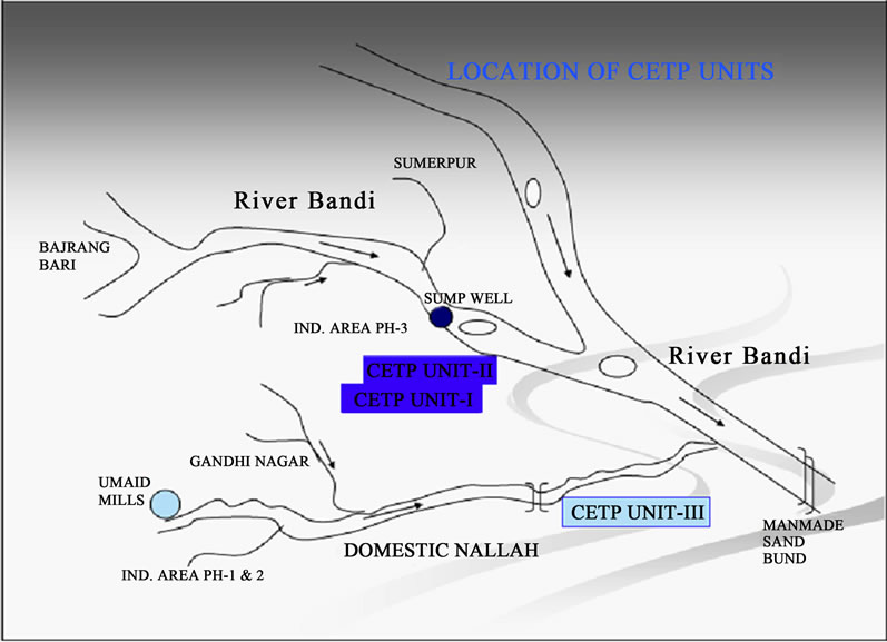
Figure 1. Pali city (source: NPC [25]).
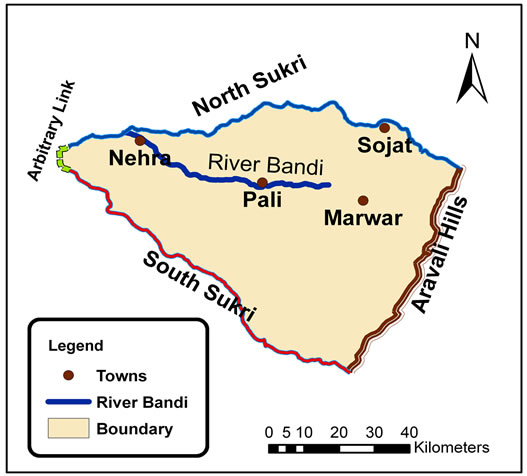
Figure 2. Study area.
verify the alignment with the physical features and the same reveals a good alignment. The study area map imposed on Google map is shown in Figure 3 [26]. Thus, an area of 5135 km2 along the river Bandi was identified as study area in order to study the impact of textile industries in an around Pali city.
108 wells located in and around the study area (Figure 4) having consistent records were selected and on the basis of historical water level data of these wells, water level surfaces for monsoon and non-monsoon seasons were prepared for the period from 1999 to 2003 by Inverse distance weighted (IDW) interpolation method. Cell size of 360 × 360 m was chosen for output image while carrying out interpolation. Figure 4 also shows the raster image of groundwater surface, of pre monsoon 2003.
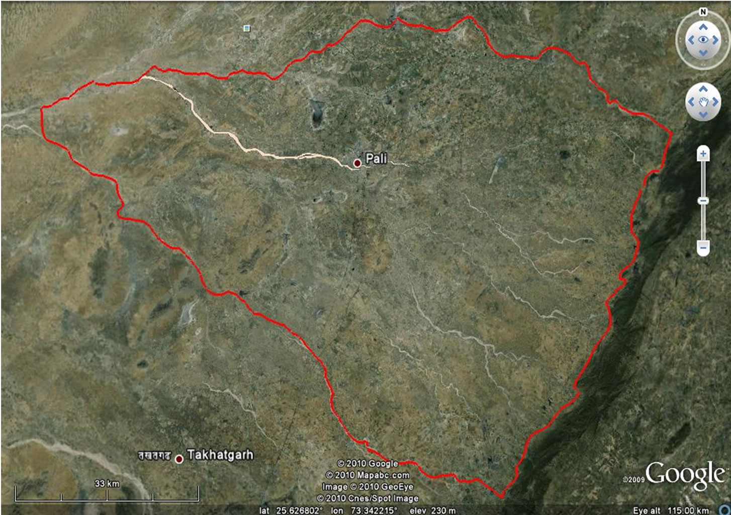
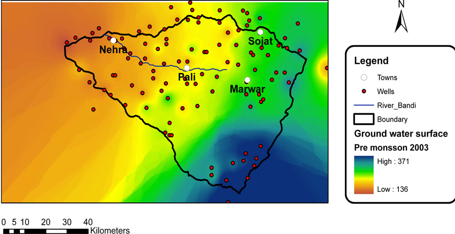
Figure 4. Map showing monitoring wells and groundwater surface, pre monsoon 2003.
Hydrostratigraphic map of the study area was prepared with the help of 28 exploratory well logs obtained from Central Groundwater Board and State Groundwater Board. Three Hydrostratigraphic layers in the form of alluvium, granite and phylite were constructed. On the basis of borlog details, bottom elevations of all three layers were worked out. ASTER elevation values [27] were used to develop digital terrain model. Details of some of the exploratory wells in the study area along with bottom elevations for all the three layers are given in Table 1.
The borelog information was used to prepare surface layers for bottom elevation of hydrostratigraphic layers of alluvium, granite and phylite by using IDW interpolation tool. Average water level depth for all the seasons for the monitoring wells was also calculated and similarly converted into a layer by interpolation technique.
4. Methodology
As can be seen from Figure 2, the boundary on the eastern side falls on the Aravali hill range and can be assumed as a no flow boundary as no groundwater flow is expected across this physical barrier. The other boundaries of the study area are dry river beds, except a very small length on western side boundary which has been joined arbitrarily to close the study area. These boundaries have been assumed as specified flow boundaries and so a methodology is needed to compute the specified flow across various segments of these boundaries. Following methodology has been adopted for the same.
1) On the boundary, a buffer of 5 km on both inside and outside of the study area was constructed. The boundary was divided into 22 cross sections as shown in Figure 5. Three cross-sections on the west side have been numbered F1, F2 and F3. Sections on upper side are numbered clockwise from U1 to U10 and those at the bottom end are numbered clockwise L1 to L9. Some of these section numbers are shown in Figure 5. Care was taken to take more number of cross sections where sharp curvature of the boundary was encountered.
2) Then groundwater level were extracted from different pre and post monsoon water surface profiles of the years 1999 to 2003 for around 30 - 35 uniformly distributed points along each cross-section area using 3D Analyst tool.
3) In the next step, these points were plotted and 4th order polygon were fitted to each curve to determine the gradient at the exact border point as shown in Figure 6. It was observed that fitness of 4th order polygon was extremely good in all the cases. It was 0.998 for the section U4 for the post monsoon 2002 which is shown in Figure 6. From the fourth order equation, it becomes easier to obtain the gradient (dy/dx) at any point by simple differentiation. Gradient were thus calculated at the boundary point for each such profile.
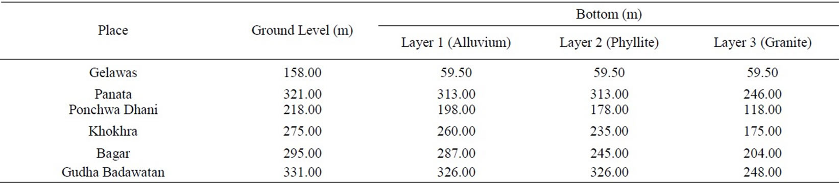
Table 1. Details of exploratory wells.
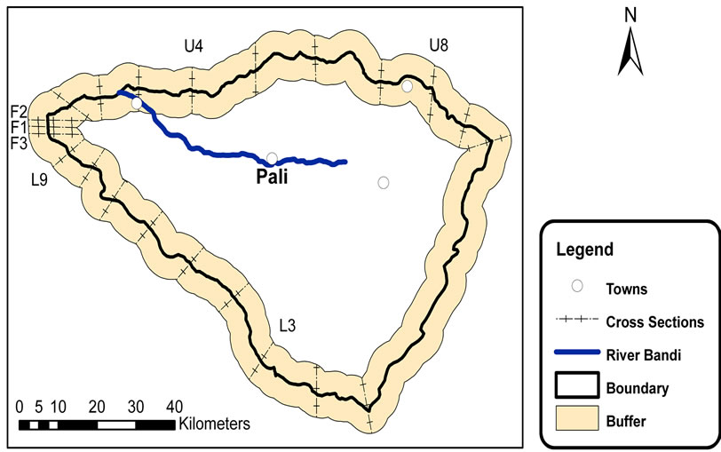
Figure 5. Map showing cross sections and points on the boundary.

Figure 6. Water level variation along section U4 for post monsoon, 2002.
4) Though the value of gradient varied between different sections, it was observed that the calculated values of gradient did not change significantly for a given crosssection between pre and post monsoon seasons and for different years. For illustration purposes, calculated values of gradient for monsoon and non monsoon seasons for different years for a few cross-sections are shown in Table 2. Gradient values were kept positive for inflow and negative for outflow into the study area boundary.
5) Accordingly, average value of gradient for each cross section was calculated by taking mean of all the calculated values of gradient for all the seasons. The average gradient values of the boundary segments so obtained for all the cross sections were then analyzed and adjacent boundary segments having almost same gradient values were identified and merged. By this method, the entire boundary was regrouped into 8 boundary segments and average values of gradients were calculated for theses 8 boundary segments based on the average values of individual line segments. These segments and average values of gradients are shown in Figure 7. Eastern boundary is shown with value of “0” (no flow).
6) Five points were selected on each boundary segment as shown in Figure 7 and values for ground level, bottom elevations of hydrostratigraphic layers and average water depth were extracted for these points from the respective layers. Thus, details of 40 boundary points selected on 8 boundary segments were tabulated. These values were then used to calculate equivalent horizontal hydraulic conductivity of the three-layered aquifer system at every point. Then the Darcy’s law was used to calculate inflow/outflow per m length of the boundary at each point. Average value of discharge was then calculated for each segment and was multiplied by the segment length to calculate gross inflow/outflow from each segment which is shown in Table 3.
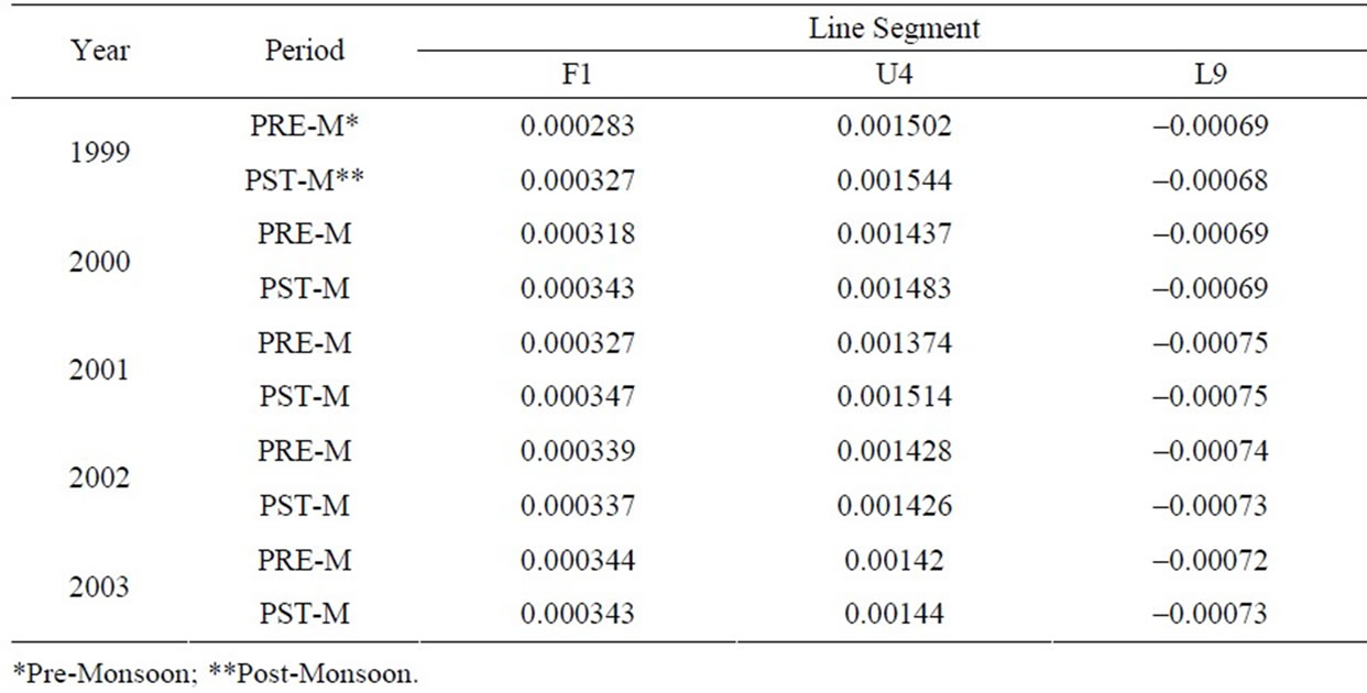
Table 2. Calculated values of gradients for typical line segments.
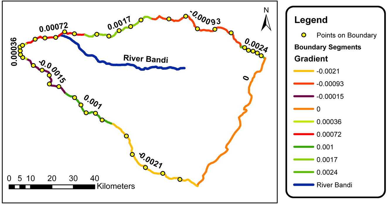
Figure 7. Final water level gradient at different boundary segments.
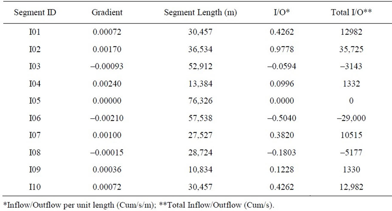
Table 3. Values of inflow/outflow for each boundary segment.
5. Results and Conclusions
The paper presented here demonstrates a GIS based methodology to work out inflow/outflow across boundary of a study area in situations where it is not possible to identify no flow boundaries in the vicinity of the study area. This methodology has been adopted for calculating the inflow/outflow along such boundaries for the groundwater model being developed for study area in Pali district.
The methodology is simple and is based on the assumption that the groundwater level gradients do not change significantly for different seasons and amongst different years that has been validated in the present groundwater model being developed for Pali district, Rajasthan, India.
In the present study, the study area boundary was divided in to 9 segments and values of flow gradients were calculated at each boundary segment. Typically the gradients were low. Maximum magnitude (0.0024) was at segment No. 4. Net flow rate varied from –0.5040 to 0.9778.
Methodology is based on utilizing a sequence of GIS based tools to calculate gradient across the boundary and then to use the Darcy’s law to calculate the flow across such boundaries.
REFERENCES
- M. Sophocleous, “Interactions between Groundwater and Surface Water: The State of the Science,” Hydrogeology, Vol. 10, No. 1, 2002, pp. 52-67. doi:10.1007/s10040-001-0170-8
- M. Sophocleous, “From Safe Yield to Sustainable Development of Water Resources—The Kansas Experience,” Hydrology, Vol. 235, No. 1-2, 2000, pp. 27-43. doi:10.1016/S0022-1694(00)00263-8
- R. K. Mall, A. Gupta, R. Singh, R. S. Singh and L. S. Rathore, “Water Resources and Climate Change: An Indian Perspective,” Current Science, Vol. 90, No. 12, 2006, pp. 1610-1626.
- M. Rodell, I. Velicogna and J. S. Famiglietti, “Satellite-Based Estimates of Groundwater Depletion in India,” Nature, Vol. 460, 2009, pp. 999-1002. doi:10.1038/nature08238
- J. Rathore, S. Jain, S. Sharma, V. Choudhary and A. Sharma, “Groundwater Quality Assessment at Pali, Rajasthan (India),” Journal of Environmental Science and Engineering, Vol. 51, No. 4, 2009, pp. 269-272.
- A. K. Meena, C. Rajagopal, P. Bansal and P. N. Nagar, “Analysis of Water Quality Characteristics in Selected Areas of Pali District in Rajasthan,” Indian Journal of Environmental Protection, Vol. 29, No. 11, 2009, pp. 1011-1016.
- V. Singhal, R. Goyal, S. Khendelwal, N. Kaul and A. B. Gupta, “Ground Water Pollution at PaliHistorical Perceptive and Future Research Needs,” Proceedings 14th National Symposium on Hydrology with Focal Theme on Management of Water Resources under Drought Situation, MNIT Jaipur, 21-22 December 2010.
- K. Spitz and J. Moreno, “A Practical Guide to Groundwater and Solute Transport Modeling,” John Wiley and Sons Inc., New York, 1996.
- J. Randall Hunt, M. P. Anderson and K. A. Victor, “Improving a Complex Finite-Difference Groundwater Flow Model through the Use of an Analytic Element Screeing Model,” Groundwater, Vol. 36, No. 6, 1998, pp. 1011- 1017. doi:10.1111/j.1745-6584.1998.tb02108.x
- M. P. Anderson and W. W. Woessner, “Applied Groundwater Modeling—Simulation of Flow and Advective Transport,” Academic Press, San Diego, 1992, p. 381.
- P. B. Bedient, H. Rifai and C. Newell, “Groundwater Contamination Transport and Remediation,” PTR Prentice Hall, Englewood Cliffs, 1994.
- T. C. Winter, “Relation of Streams, Lakes, and Wetlands to Groundwater Flow Systems,” Hydrogeology, Vol. 7, No. 1, 1999, pp. 28-45. doi:10.1007/s100400050178
- W. W. Woessner, “Stream and Fluvial Plain Groundwater Interactions: Rescaling Hydrogeologic Thought,” Groundwater, Vol. 38, No. 3, 2000, pp. 423-429. doi:10.1111/j.1745-6584.2000.tb00228.x
- M. Brunke and T. Gonser, “The Ecological Significance of Exchange Processes between Rivers and Ground-Water,” Freshwater Biology, Vol. 37, No. 1, 1997, pp. 1-33. doi:10.1046/j.1365-2427.1997.00143.x
- D. W. Watkins, D. C. McKinney, D. R. Maidment and M.-D. Lin, “Use of Geographic Information Systems in Ground-Water Flow Modeling,” Journal of Water Resources Planning and Management, ASCE, Vol. 122, No. 2, 1996, pp. 88-96. doi:10.1061/(ASCE)0733-9496(1996)122:2(88)
- R. Gogu, G. Carabin, V. Hallet, V. Peters and A. Dassargues, “GIS-Based Hydrogeological Databases and GroundWater Modelling,” Hydrogeology, Vol. 9, No. 6, 2001, pp. 555-569. doi:10.1007/s10040-001-0167-3
- W. R. Talbot and K. E. Kolm, “Conceptualization and Characterization and Numerical Simulation of Hydrogeologic System Using GIS. A Site Specific Case Study at NPL Site near Cheyenne, Wyoning,” Association of English Geology Programme Abstract, San Antonio, 9-16 October 1993, p. 74.
- K. E. Kolm, “Conceptualization and Characterization of Groundwater Systems Using Geographical Information System,” Engineering Geology, Vol. 42, No. 2-3, 1996, pp. 111-118. doi:10.1016/0013-7952(95)00072-0
- C. Bhuiyan, Ramesh P. Singh and W. A. Flügel, “Modeling of Ground Water Recharge-Potential in the Hardrock Aravalli Terrain, India: A GIS Approach,” Environmental Earth Sciences, Vol. 59, No. 4, 2009, pp. 929- 938. doi:10.1007/s12665-009-0087-4
- National Productivity Council, NPC, “Study of Health and Environment Impact Due to Pollution from Textile Units in Pali, Balotra, Jasol and Bithuja,” Draft Report, New Delhi, 2007.
- Water Resources Department, Government of Rajasthan, “NIT Information,” 2011. http://waterresources.rajastha n.gov.in
- Rajasthan State Pollution Control Board, RSPCB, “Environmental Status Report, Pali,” Jaipur, 1984.
- Rajasthan State Pollution Control Board, RSPCB, “Groundwater Quality Monitoring in Problem Area of Jodhpur & Pali Districts in Rajasthan,” Jaipur, 2002.
- V. Singhal, K. Chansoria and R. Goyal, “Geo-Spatial Analysis of Surface and Groundwater Quality along Bandi River, Pali,” Proceedings of National Conference on Hydraulics, Water Resources and Environment, Jaipur, 15-16 December 2008, pp. 134-143.
- National Productivity Council, NPC, “Study of Health and Environment Impact Due to Pollution from Textile Units in Pali, Balotra, Jasol and Bithuja,” Final Report, 2010.
- Google, “Google Earth,” 2010. http://earth.google.com
- Earth Remote Sensing Data Analysis Center (ERSDAC), “ASTER GDEM,” 2010. http://www.gdem.aster.ersdac. or.jp