Journal of Software Engineering and Applications
Vol.7 No.1(2014), Article ID:42100,11 pages DOI:10.4236/jsea.2014.71005
Multi-Threshold Algorithm Based on Havrda and Charvat Entropy for Edge Detection in Satellite Grayscale Images
1Department of Mathematics, Faculty of Science, Fayoum University, Al Fayoum, Egypt; 2Assistant Professor of Computer Science, Taif University, Taif, KSA; 3Department of Mathematics, Faculty of Science, Aswan University, Aswan, Egypt.
Email: mas06@fayoum.edu.eg
Copyright © 2014 Mohamed A. El-Sayed, Hamida A. M. Sennari. This is an open access article distributed under the Creative Commons Attribution License, which permits unrestricted use, distribution, and reproduction in any medium, provided the original work is properly cited. In accordance of the Creative Commons Attribution License all Copyrights © 2014 are reserved for SCIRP and the owner of the intellectual property Mohamed A. El-Sayed, Hamida A. M. Sennari. All Copyright © 2014 are guarded by law and by SCIRP as a guardian.
Received November 27th, 2013; revised December 25th, 2013; accepted January 2nd, 2014
KEYWORDS
Multi-Threshold; Edge Detection; Measure Entropy; Havrda & Charvat’s Entropy
ABSTRACT
Automatic edge detection of an image is considered a type of crucial information that can be extracted by applying detectors with different techniques. It is a main tool in pattern recognition, image segmentation, and scene analysis. This paper introduces an edge-detection algorithm, which generates multi-threshold values. It is based on non-Shannon measures such as Havrda & Charvat’s entropy, which is commonly used in gray level image analysis in many types of images such as satellite grayscale images. The proposed edge detection performance is compared to the previous classic methods, such as Roberts, Prewitt, and Sobel methods. Numerical results underline the robustness of the presented approach and different applications are shown.
1. Introduction
Edge detection is a very important tool used in many applications of image processing to obtain information from the frames as a preparatory step to feature extraction and object segmentation. This phase detects outlines of an object and boundaries between objects and the background in the image [1]. The detection results benefit applications such as optical character recognition [2], infrared gait recognition [3,4], automatic target recognition [5], detection of video changes [6], and medical image applications [7].
Edge detection concerns localization of abrupt changes in the gray level of an image [8]. Edge detection can be defined as the boundary between two regions separated by two relatively distinct gray level properties [9]. The causes of the region dissimilarity may be due to some factors such as the geometry of the scene, the radio metric characteristics of the surface, the illumination and so on [10]. An effective edge detector reduces a large amount of data but still keeps most of the important feature of the image. Edge detection refers to the process of locating sharp discontinuities in an image [11,12].
Many operators have been introduced in the literature, for example, Roberts, Sobel and Prewitt [13-17]. Edges are mostly detected using either the first derivatives, called gradient, or the second derivatives, called Laplacien. Laplacien is more sensitive to noise since it uses more information because of the nature of the second derivatives.
Most of the classical methods for edge detection based on the derivative of the pixels of the original image are Gradient operators, Laplacien and Laplacien of Gaussian (LOG) operators [10]. Gradient based edge detection methods, such as Roberts, Sobel and Prewitts, have used two linear filters to process vertical edges and horizontal edges separately to approximate first-order derivative of pixel values of the image. Marr and Hildreth achieved this by using the Laplacien of a Gaussian (LoG) function as a filter [18]. To solve these problems, the study proposed a novel approach based on information theory, which is entropy-based thresholding. The proposed method is to decrease the computation time compared with Canny and LoG method. The results were very good compared with the well-known Roberts, Prewitt, and Sobel gradient results.
The outline of the paper is as follows. In Section 2, we have presented the classical edge detection methods that related to the paper. Image thresholding based on Havrda & Charvat’s entropy is presented in Section 3. Section 4 describes the edge detection that was based on entropy. Section 5 illustrates the multi-threshold algorithm based on Havrda and Charvat entropy for edge detection. In Section 6, we have presented the effectiveness of proposed algorithm in the case of satellite grayscale images, and also we compared the results of the algorithm with several leading edge detection methods such as Roberts, Prewitt, and Sobel methods in the same section. Conclusions are presented in Section 7.
2. Classical Edge Detection Methods
Five most frequently used edge detection methods are used for comparison. These are: Gradient operators (Roberts, Prewitt, Sobel), Laplacian of Gaussian (LoG or Marr-Hildreth) and Gradient of Gaussian (Canny) edge detections [19,20]. People which would like to read about this subject are referred to [21-23] evaluation studies of edge detection algorithms according to different criteria. The details of methods as follows,
2.1. Roberts Edge Detector
The Roberts Cross operator performs a simple, quick to compute, 2-D spatial gradient measurement on an image as shown in Figure 1. It thus highlights regions of high spatial frequency which often correspond to edges. In its most common usage, the input to the operator is a grayscale image, as is the output. Pixel values at each point in the output represent the estimated absolute magnitude of the spatial gradient of the input image at that point [20].
2.2. Prewitt Edge Detector
The Prewitt edge detector is an appropriate way to estimate the magnitude and orientation of an edge. Although differential gradient edge detection needs a rather time consuming calculation to estimate the orientation from the magnitudes in the x and y-directions, the compass edge detection obtains the orientation directly from the kernel with the maximum response. The Prewitt operator is limited to 8 possible orientations, however experience shows that most direct orientation estimates are not much more accurate. This gradient based edge detector is estimated in the 3 × 3 neighbourhood for eight directions as shown in Figure 2. All the eight convolution masks are calculated. One convolution mask is then selected, namely that with the largest module [20].
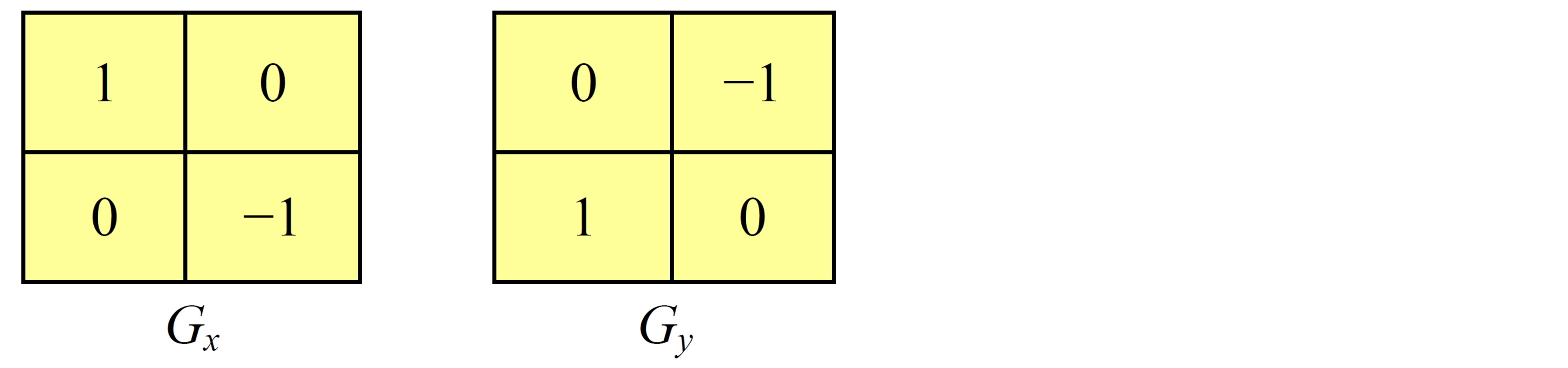
Figure 1. Roberts gradient estimation operator.
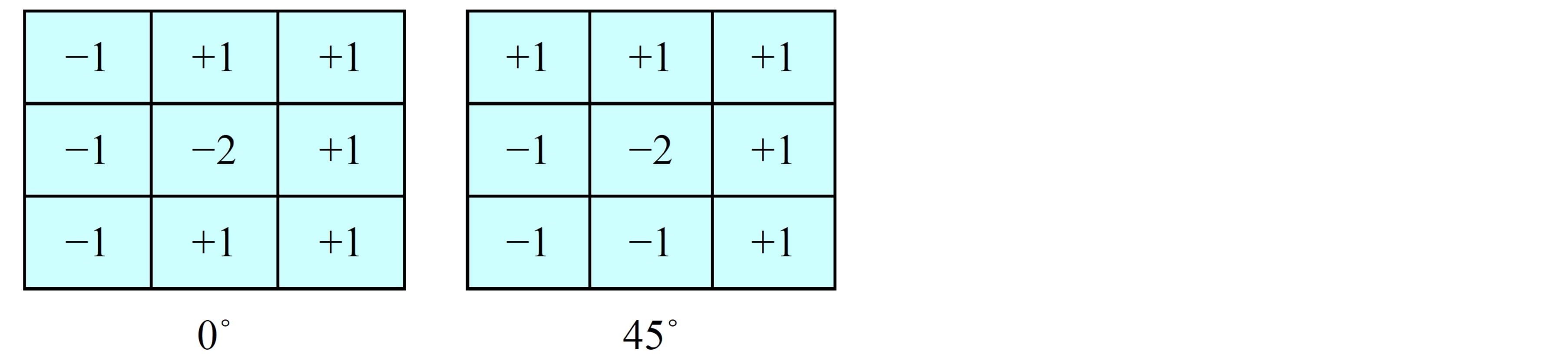
Figure 2. Prewitt gradient estimation operator.
2.3. Sobel Edge Detector
The operator consists of a pair of 3 × 3 convolution kernels as shown in Figure 3. One kernel is simply the other rotated by 90˚.
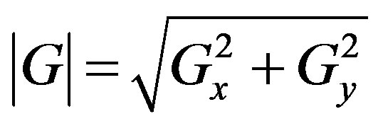
These kernels are designed to respond maximally to edges running vertically and horizontally relative to the pixel grid, one kernel for each of the two perpendicular orientations. The kernels can be applied separately to the input image, to produce separate measurements of the gradient component in each orientation (call these Gx and Gy). These can then be combined together to find the absolute magnitude of the gradient at each point and the orientation of that gradient [20]. The gradient magnitude is given by:
Typically, an approximate magnitude is computed using:

which is much faster to compute.
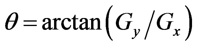
The angle of orientation of the edge (relative to the pixel grid) giving rise to the spatial gradient is given by:
2.4. Canny Edge Detector
This edge detector is due to J.F. Canny [19] (a recursive implementation of this algorithm was presented in [24]). In his work Canny specified three main criteria for the performance of edge detectors: First criteria, (low error rate) minimum number of false negatives and false positives. Second criteria, good localization, report edge location at correct position. In other words, the distance between the edge pixels as found by the detector and the actual edge is to be at a minimum. A third criterion is to have only one response to a single edge. In order to implement the canny edge detector algorithm, a series of steps must be followed.
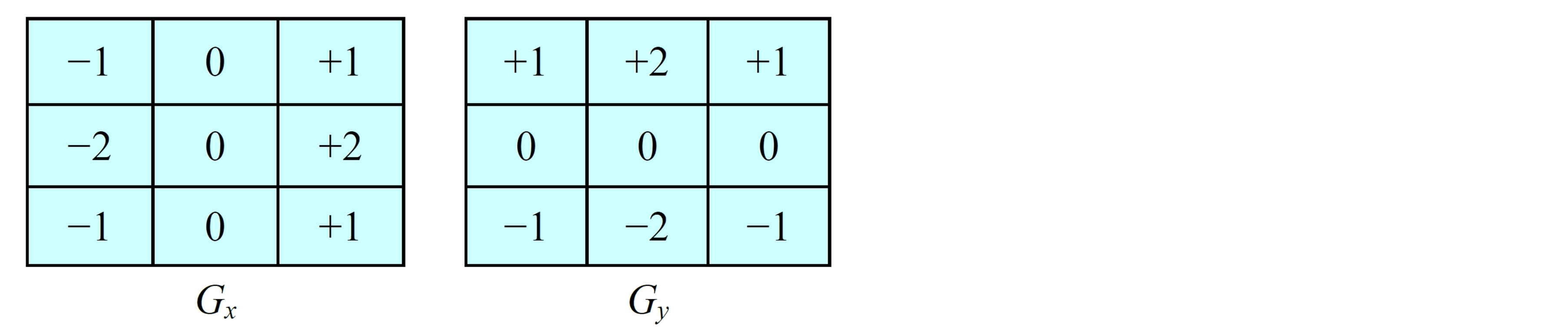
Figure 3. Sobel gradient estimation operator.
Step 1: The first step is to filter out any noise in the original image before trying to locate and detect any edges. It uses a filter based on a Gaussian (bell curve), where the raw image is convolved with a Gaussian filter. The result is a slightly blurred version of the original which is not affected by a single noisy pixel to any sig nificant degree. The Gaussian mask used in my implementation is shown in Figure 4 with σ = 1.4.
Step 2: After smoothing the image and eliminating the noise, the next step is to find the edge strength by taking the gradient of the image using the Sobel operator uses a pair of 3 × 3 convolution masks. The approximate gradient magnitude is given by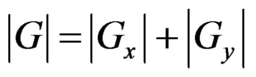 .
.
Step 3: Finding the edge direction is trivial once the gradient in the x and y directions are known. However, you will generate an error whenever sumX is equal to zero. So in the code there has to be a restriction set whenever this takes place. Whenever the gradient in the x direction is equal to zero, the edge direction has to be equal to 90 degrees or 0 degrees, depending on what the value of the gradient in the y-direction is equal to. If Gy has a value of zero, the edge direction will equal 0 degrees. Otherwise the edge direction will equal 90 degrees. The formula for finding the edge direction is just: 
Step 4: Once the edge direction is known, the next step is to relate the edge direction to a direction that can be traced in an image. So if the pixels of a 5 × 5 image are aligned as follows in Figure 5.
Then, it can be seen by looking at pixel “a”, there are only four possible directions when describing the surrounding pixels, 0 degrees (in the horizontal direction), 45 degrees (along the positive diagonal), 90 degrees (in the vertical direction), or 135 degrees (along the negative diagonal). So now the edge orientation has to be resolved into one of these four directions depending on which direction it is closest to (e.g. if the orientation angle is found to be 3 degrees, make it zero degrees). Think of this as taking a semicircle and dividing it into 5 regions as shown in Figure 6.
Therefore, any edge direction falling within the range (0 to 22.5 & 157.5 to 180 degrees) is set to 0 degrees. Any edge direction falling in the range (22.5 to 67.5 degrees) is set to 45 degrees. Any edge direction falling in the range (67.5 to 112.5 degrees) is set to 90 degrees. And finally, any edge direction falling within the range (112.5 to 157.5 degrees) is set to 135 degrees.
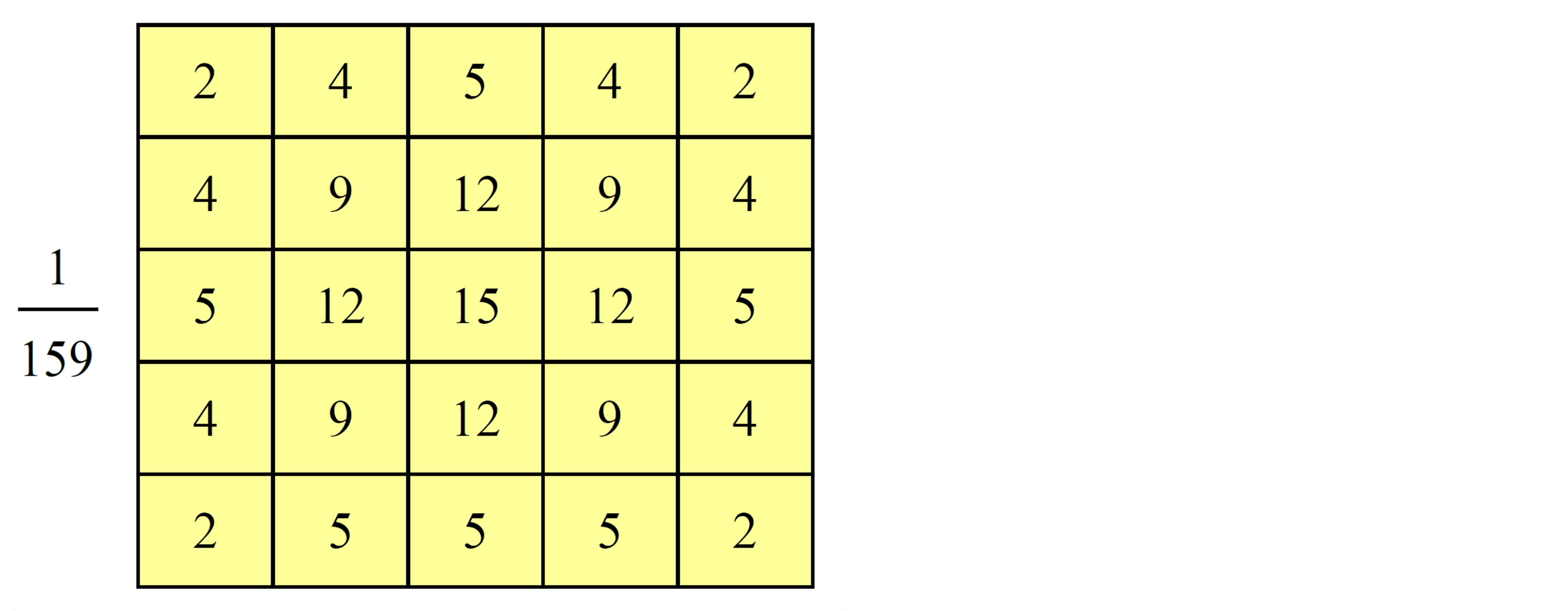
Figure 4. Discrete approximation to Gaussian function with σ = 1.4.
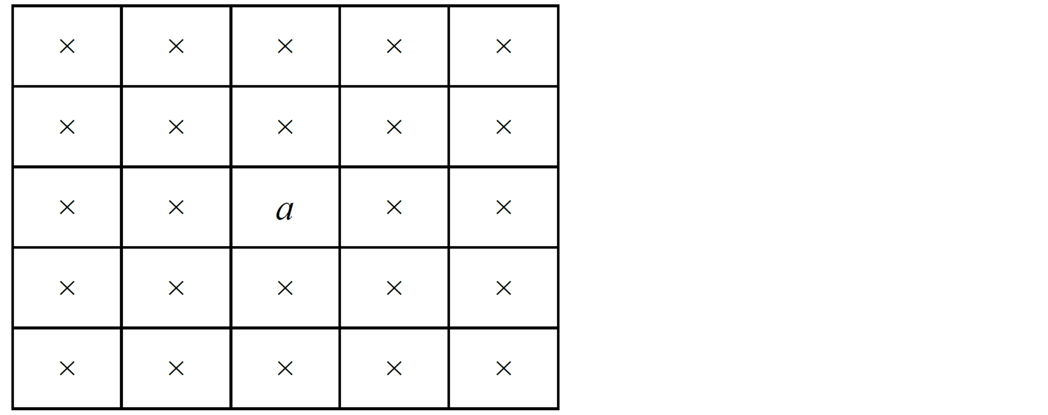
Figure 5. The pixel “a” and the possible directions.
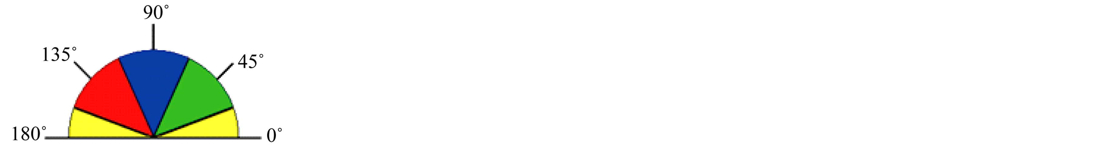
Figure 6. The range of edge direction in the five regions.
Step 5: After the edge directions are known, nonmaximum suppression now has to be applied. Nonmaximum suppression is used to trace along the edge in the edge direction and suppress any pixel value (sets it equal to 0) that is not considered to be an edge. This will give a thin line in the output image.
Step 6: Finally, hysteresis is used as a means of eliminating streaking. Streaking is the breaking up of an edge contour caused by the operator output fluctuating above and below the threshold. If a single threshold, T1 is applied to an image, and an edge has an average strength equal to T1, then due to noise, there will be instances where the edge dips below the threshold. Equally it will also extend above the threshold making an edge look like a dashed line. To avoid this, hysteresis uses 2 thresholds, a high and a low. Any pixel in the image that has a value greater than T1 is presumed to be an edge pixel, and is marked as such immediately. Then, any pixels that are connected to this edge pixel and that have a value greater than T2 are also selected as edge pixels. If you think of following an edge, you need a gradient of T2 to start but you don’t stop till you hit a gradient below T1.
3. Havrda & Charvat’s Entropy
Regarding the statistical approach for describing texture, one of the simplest computational approaches is to use statistical moments of the gray level histogram of the image. The image histogram carries important information about the content of an image and can be used for discriminating the abnormal tissue from the local healthy background. Considering the gray level histogram
 where
where  is the number of distinct gray levels in the ROI (region of interest). If n is the total number of pixels in the region, then the normalized histogram of the ROI is the set
 , where
 . The source symbol probabilities is
 . This set of probabilities must satisfy the condition,
 . The average information per source output, denoted S(H) [25], Shannon entropy may be described as:
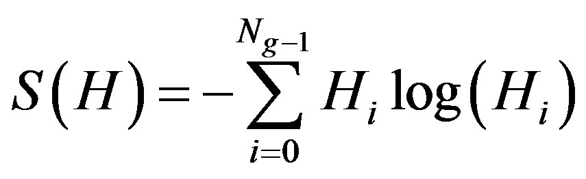 (2)
(2)
If we consider that a system can be decomposed in two statistical independent subsystems A and B, the Shannon entropy has the extensive property (additivity)
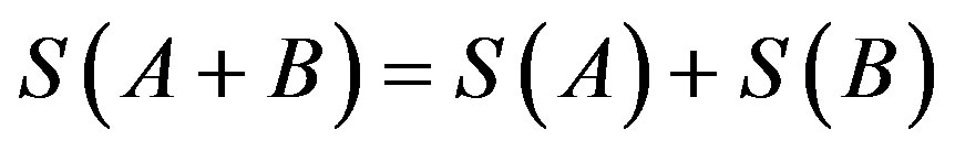 , this formalism has been shown to be restricted to the Boltzmann-Gibbs-Shannon (BGS) statistics.
However, for non-extensive systems, some kind of extension appears to become necessary. Havrda & Charvat’s [26,27] has proposed a generalization of the BGS statistics which is useful for describing the thermo statistical properties of non-extensive systems. It is based on a generalized entropic form,
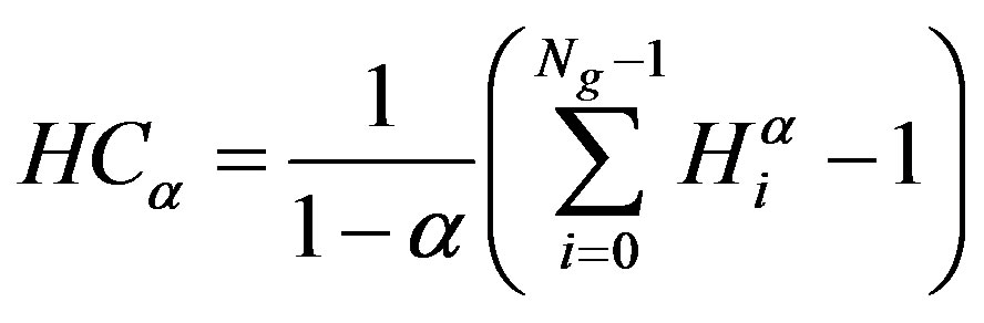 (3)
(3)
where the real number  is a entropic index that characterizes the degree of non-extensivity. This expression recovers to BGS entropy in the limit
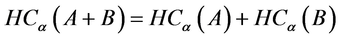
 . Havrda & Charvat’s entropy has a non-extensive property for statistical independent systems, defined by the following rule [28]:
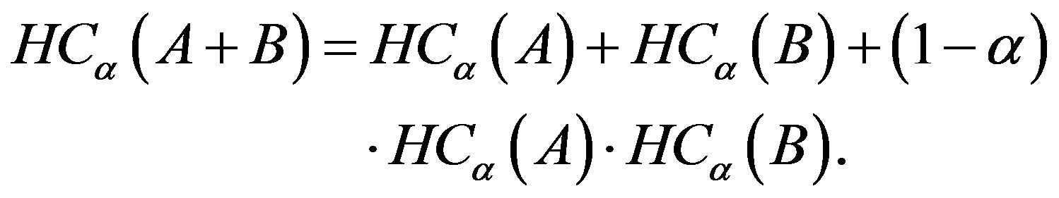 (4)
(4)
Similarities between Boltzmann-Gibbs and Shannon entropy forms give a basis for possibility of generalization of the Shannon’s entropy to the Information Theory. This generalization can be extended to image processing areas, specifically for the image segmentation, applying Havrda & Charvat’s entropy to threshold images, which have non-additive information content.
Considering  in the pseudo-additive formalism of Equation (4), three different entropies can be defined with regard to different values of
 .
.
For , the Havrda & Charvat’s entropy becomes a “sub extensive entropy” where:
 (5)
(5)
For , the Havrda & Charvat’s entropy reduces to an standard “extensive entropy” where:
 (6)
(6)
For , the Havrda & Charvat’s entropy becomes a “super extensive entropy” where:
 (7)
(7)
Let f(x, y) be the gray value of the pixel located at the point (x, y). In a digital image
 of size M × N, let the histogram be h(a) for
  with f as the amplitude (brightness) of the image at the real coordinate position (x, y). For the sake of convenience, we denote the set of all gray levels
  as G. Global threshold selection methods usually use the gray level histogram of the image. The optimal threshold t* is determined by optimizing a suitable criterion function obtained from the gray level distribution of the image and some other features of the image.
Let t be a threshold value and B = {b0, b1} be a pair of binary gray levels with  Typically b0 and b1 are taken to be 0 and 1, respectively. The result of thresholding an image function f(x, y) at gray level t is a binary function
  such that
  if
if  otherwise,
 . In general, a thresholding method determines the value t* of t based on a certain criterion function. If t* is determined solely from the gray level of each pixel, the thresholding method is point dependent [25].
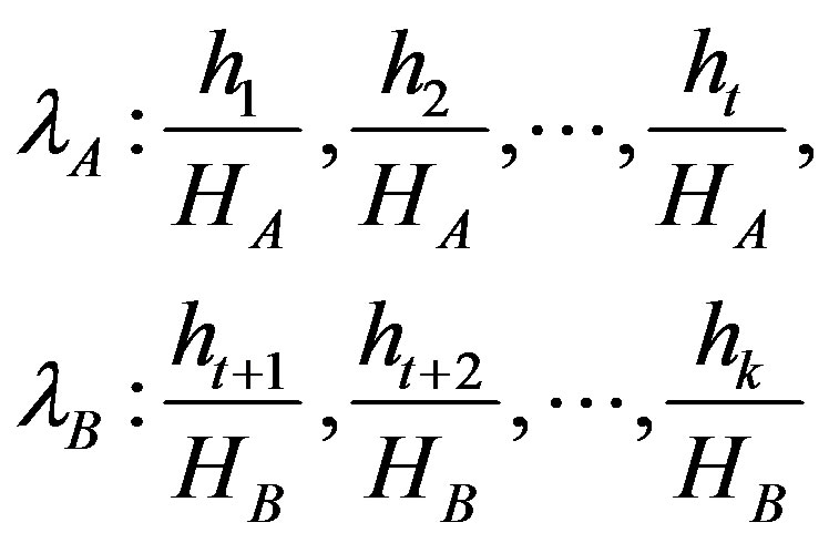
Let 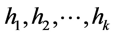 be the probability distribution for an image with k gray-levels. From this distribution, we derive two probability distributions, one for the object (class A) and the other for the background (class B), given by:
 (8)
(8)
and where
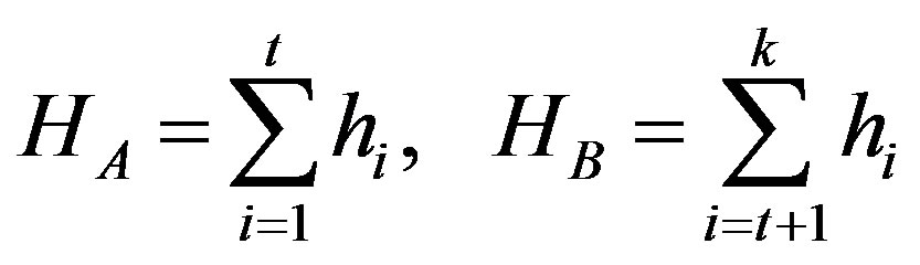 (9)
(9)
The Havrda & Charvat’s entropy of order q for each distribution is defined as:
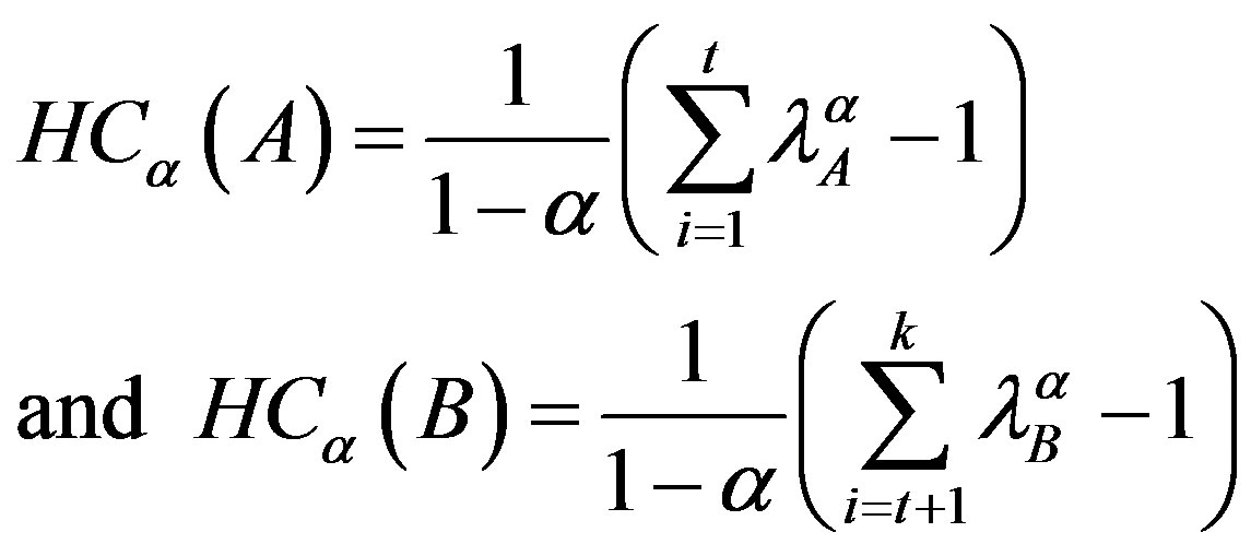 (10)
(10)
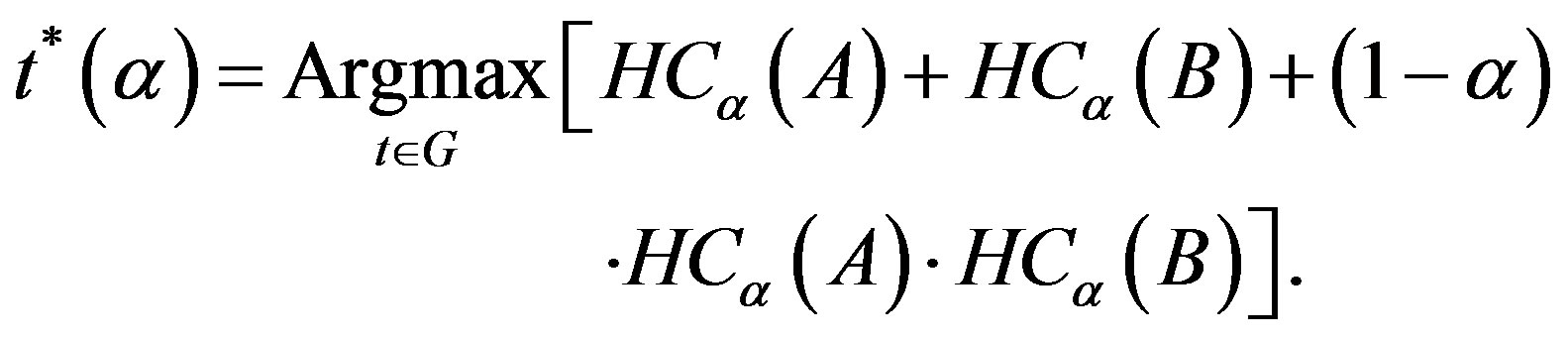
The Havrda & Charvat’s entropy  is parametrically dependent upon the threshold value t for the foreground and background. It is formulated as the sum each entropy, allowing the pseudo-additive property, defined in Equation (3). We try to maximize the information measure between the two classes (object and background). When
  is maximized, the luminance level t that maximizes the function is considered to be the optimum threshold value.
 (11)
(11)
In the proposed scheme, first create a binary image by choosing a suitable threshold value using Havrda & Charvat’s entropy. The technique consists of treating each pixel of the original image and creating a new image, such that  if
if  otherwise,
  for every
 ,
, .
.
When , the threshold value in Equation (3), equals to the same value found by Shannon’s method. Thus this proposed method includes Shannon’s method as a special case. The following expression can be used as a criterion function to obtain the optimal threshold at
 .
.
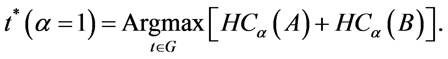 (12)
(12)
The Havrda_Charvat_T procedure to select suitable threshold value t* with  for grayscale image f can now be described as follows:
Procedure Havrda_Charvat_T,
Input: An image f of size r × c, and .
.
Output: optimal threshold t* of f.
Begin 1. Let f(x, y) be the original gray value of the pixel at the point (x, y), x = 1.. r, y = 1.. c.
2. Calculate the probability distribution 0 ≤ hi ≤ 255.
3. For all t {0, 1, …, 255}i. Calculate
 ,
,  ,
,  , and
, and  using Equations (8) and (9).
ii. Find optimum threshold value t*, such that

End.
The technique consists of treating each pixel of the original image and creating a new image, such that  if
if  otherwise,
  for every
 ,
, .
.
4. Detecting of the Edges
We will use the usual masks for detecting the edges [29]. A spatial filter mask may be defined as a matrix w of size m × n. Assume that m = 2μ + 1 and n = 2ρ + 1, where μ, ρ are nonzero positive integers. For this purpose, smallest meaningful size of the mask is 3 × 3. Such mask coefficients, showing coordinate arrangement as Figure 7(a). Image region under the above mask is shown as Figure 7(b).
In order to edge detection, firstly classification of all pixels that satisfy the criterion of homogeneousness, and detection of all pixels on the borders between different homogeneous areas. In the proposed scheme, first create a binary image by choosing a suitable threshold value using Havrda & Charvat entropy. Window is applied on the binary image. Set all window coefficients equal to 1 except centre, centre equal to × as shown in Figure 8.
Move the window on the whole binary image and find the probability of each central pixel of image under the window. Then, the entropy of each central pixel of image under the window is calculated as S(CPix) = –pcln(pc). Where, pc is the probability of central pixel CPix of binary image under the window. When the probability of central pixel, pc = 1, then the entropy of this pixel is zero. Thus, if the gray level of all pixels under the window homogeneous, pc = 1 and S = 0. In this case, the central pixel is not an edge pixel. Other possibilities of entropy of central pixel under window are shown in Table 1.
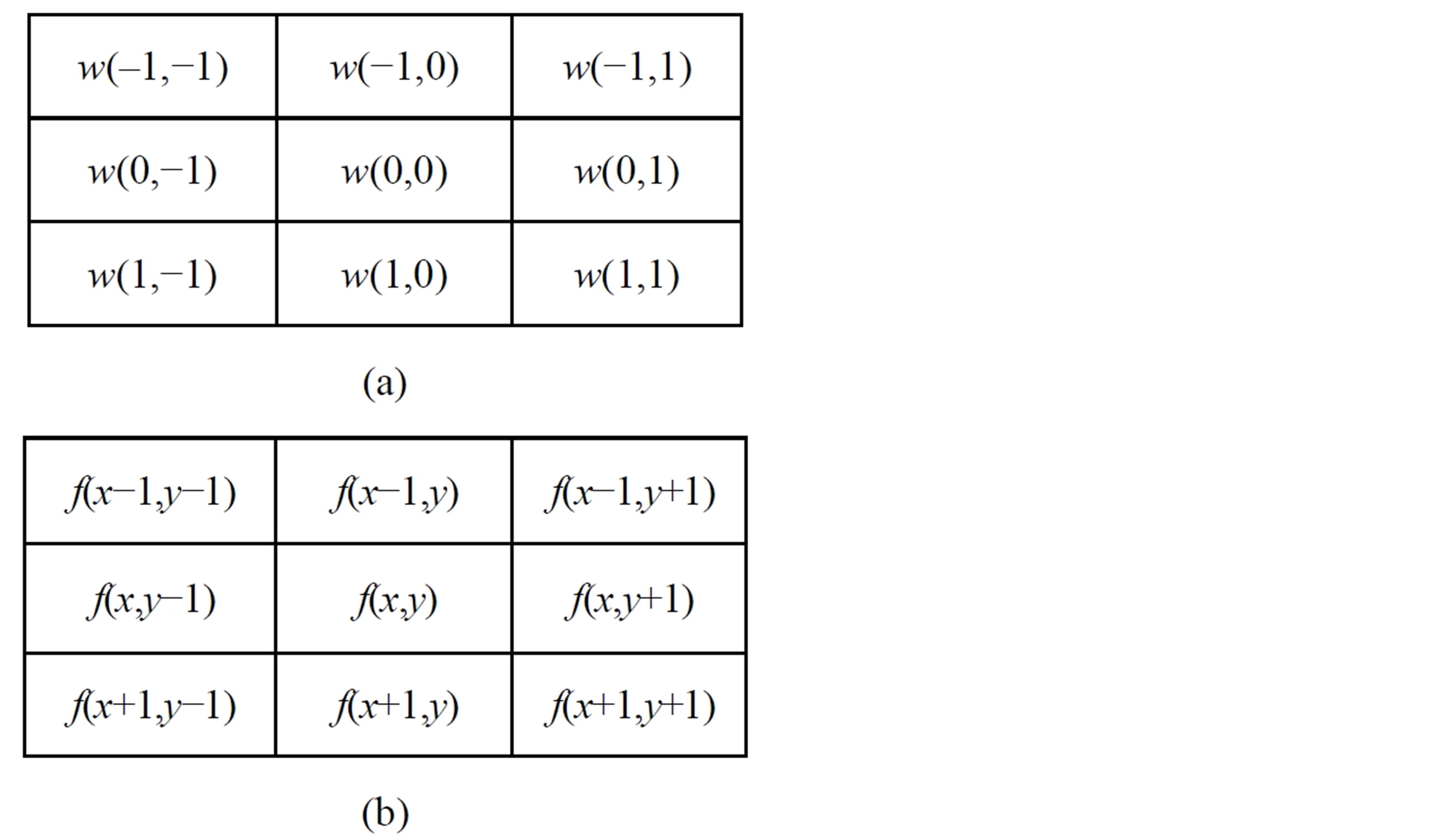
Figure 7. Coordinate arrangement and image region under 3 × 3 mask.
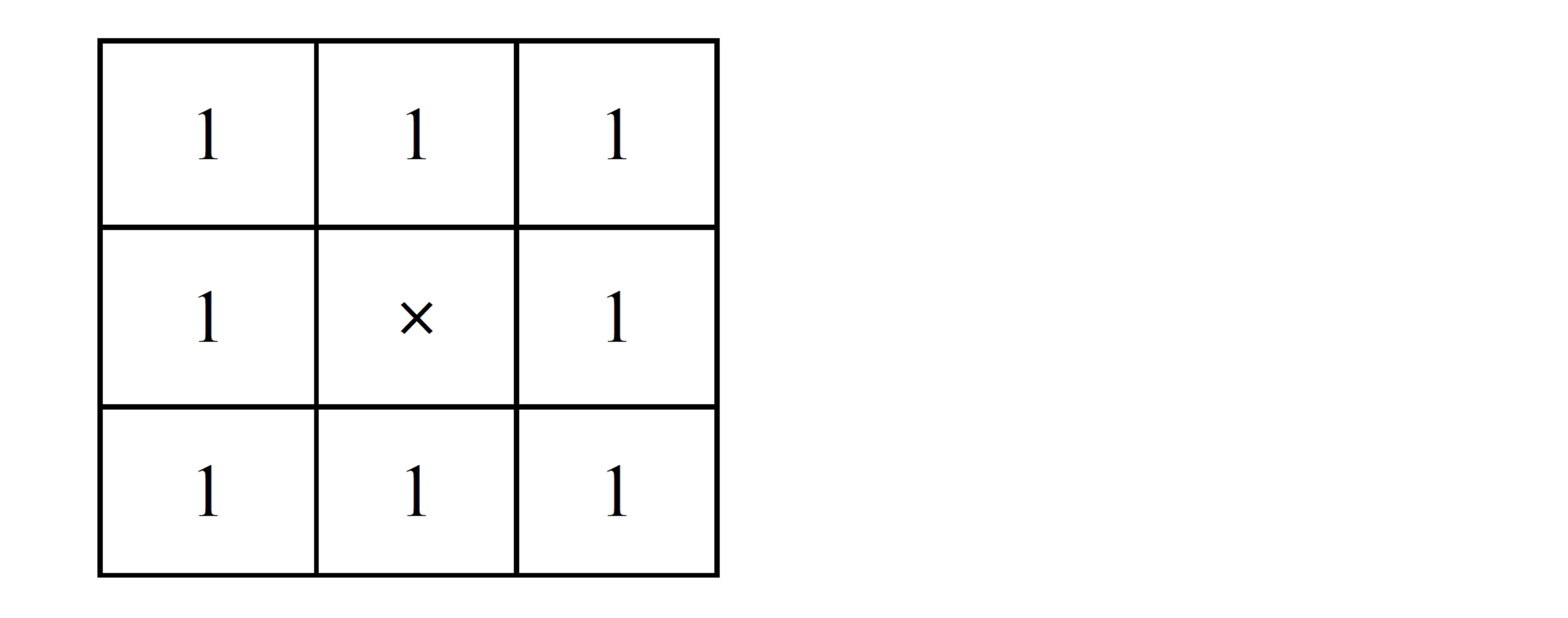
Figure 8. Window coefficients of 3 × 3 mask.
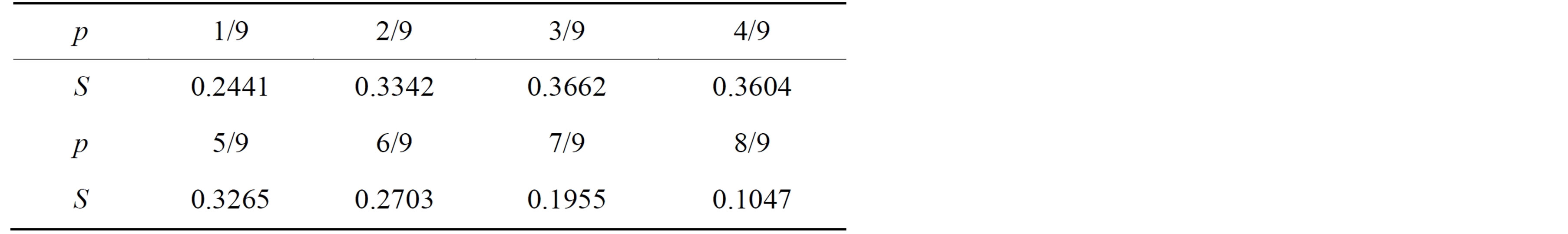
Table 1. p and S of central under window.
In cases pc = 8/9, and pc = 7/9, the diversity for gray level of pixels under the window is low. So, in these cases, central pixel is not an edge pixel. In remaining cases, pc ≤ 6/9, the diversity for gray level of pixels under the window is high. The complete algorithm can now be described as follows:
Algorithm HCEdgeDetection;
Input: A grayscale image A (M × N).
Output: The edge detection image g.
Begin
1. Select suitable t*, α, using Havrda_Charvat_T procedure.
2. Create a binary image:
If f(x, y) ≤ t* α) then f (x,y) = 0 Else f(x, y) = 1.
3. Create a mask w, with dimensions m × n:
Normally, m = n = 3. μ = (m−1)/2 and ρ = (n−1)/2.
4. For all 1 ≤ x≤ M and 1 ≤ y ≤ N:
Find g an output image by set g = f.
5. For all ρ + 1≤ y ≤ N−ρ and μ + 1 ≤ x ≤ M−μchecking for edge pixels:
i. sum = 0;
ii. For all −ρ ≤ k ≤ ρ and −μ ≤ j ≤ μ:
If (f(x, y) = f (x+j, y+k)) Then Sum = sum + 1.
iii. If (sum > 6) Then g(x,y)=0 Else g(x,y) = 1.
End algorithm.
5. Proposed Algorithm
Here, the algorithm produces three different threshold values t1, t2 and t3. We use Havrda_Charvat_T procedure, to find the threshold value t1 through the entire image. Then we split the image by t1 into two grayscale parts, the object and background. Applying the Equation (11), to find the locals threshold values t2 and t3 of object and background, respectively. Independently, we apply HC EdgeDetection Procedure with threshold values t1, t2 and t3. We merge the resultant edge images to obtain the reconstructed edge image.
In order to minimize the execution time, we deal with the histogram vectors, 0, 1, ···, t1 and t1 + 1, ···, 255 of object and background parts, respectively rather than the matrices size of them.
The steps of proposed algorithm are as follows:
1- Read the grayscale level image, I = imread (‘test. tif’);
2- Calculate the histogram H with 256 elements of I;
3- Call Havrda_Charvat_T(H, α) to find the optimal threshold value, t1;
4- Divide H into two parts HLow and HHigh using t1.
5- Recall Havrda_Charvat_T(HLow, α) to find the optimal threshold value t2;
6- Recall Havrda_Charvat_T(HHigh, α) to find the optimal threshold value t3;
7- Now we have 3 values of the threshold, t2 < t1 < t3. Reconstruct bitmap image f, such that: if (Ix,y < t1 and Ix,y >= t2) or (Ix,y >= t3) then fx,y =1; end;
8- Call the procedure HCEdgeDetection(f) to find edge image g.
9- Display the image g, imshow(g);
The above procedures can be done together in the following MATLAB program:
I=imread(‘test.tif’);
alpha=0.1;
[M,N,R]=size(I);
if R==3 I=rgb2gray(I); end;
H = imhist(I);
[T1, Max1, Loc1] =
Havrda_Charvat_T(H,alpha);
HLow= H (1:Loc1-1,:);
[T2, Max2, Loc2]=
Havrda_Charvat_T(HLow,alpha);
HHigh= H (Loc1:size(H),:);
[T3, Max3, Loc3] =
Havrda_Charvat_T(HHigh,alpha);
f=zeros(M,N);
for i=1:M;
for j=1:N;
if ((I(i,j) >= T2)&(I(i,j) < T1))
|(I(i,j) >= T3) f(i,j)=1; end;
end;
end
[g]= HCEdgeDetection(f);
figure; imshow(g);
6. Results and Discussion
In order to test the method proposed in this paper and compare with the other edge detectors, common gray level test images with different resolutions and sizes are detected by Canny, LOG, Roberts, Prewitt, Sobel and the proposed method respectively. The performance of the proposed scheme is evaluated through the simulation results using MATLAB. Prior to the application of this algorithm, no pre-processing was done on the tested images (Figure 9).
The algorithm has two main phases global and local enhancement phase of the threshold values and detection phase, we present the results of implementation on these images separately. Here, we have used in addition to the original gray level function f(x, y), a function g(x, y) that is the average gray level value in a 3 × 3 neighborhood around the pixel (x, y). We use MATLAB to calculate the average time for each method at different images size by repeating 10 times for each type of image. As shown in Figure 10, the chart of the test images and the average of run time for the classical methods and proposed scheme.
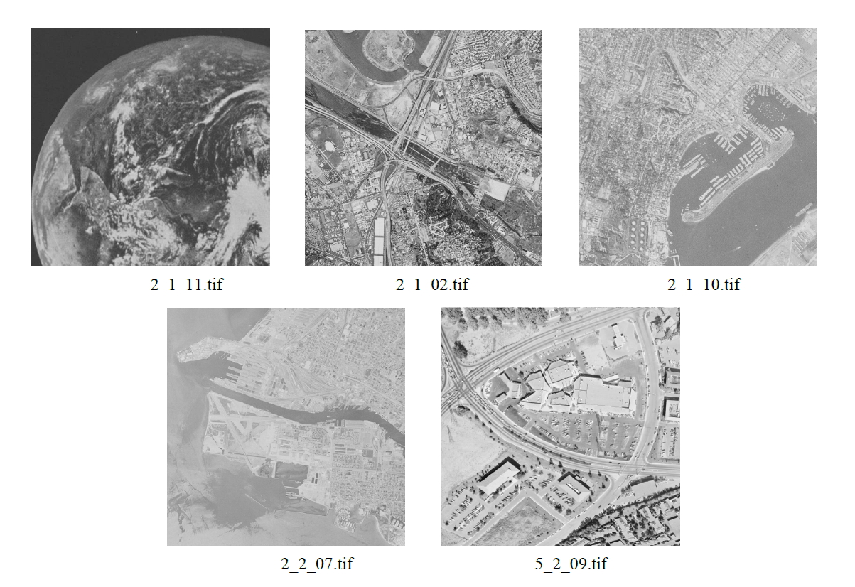
Figure 9. Samples of test images.
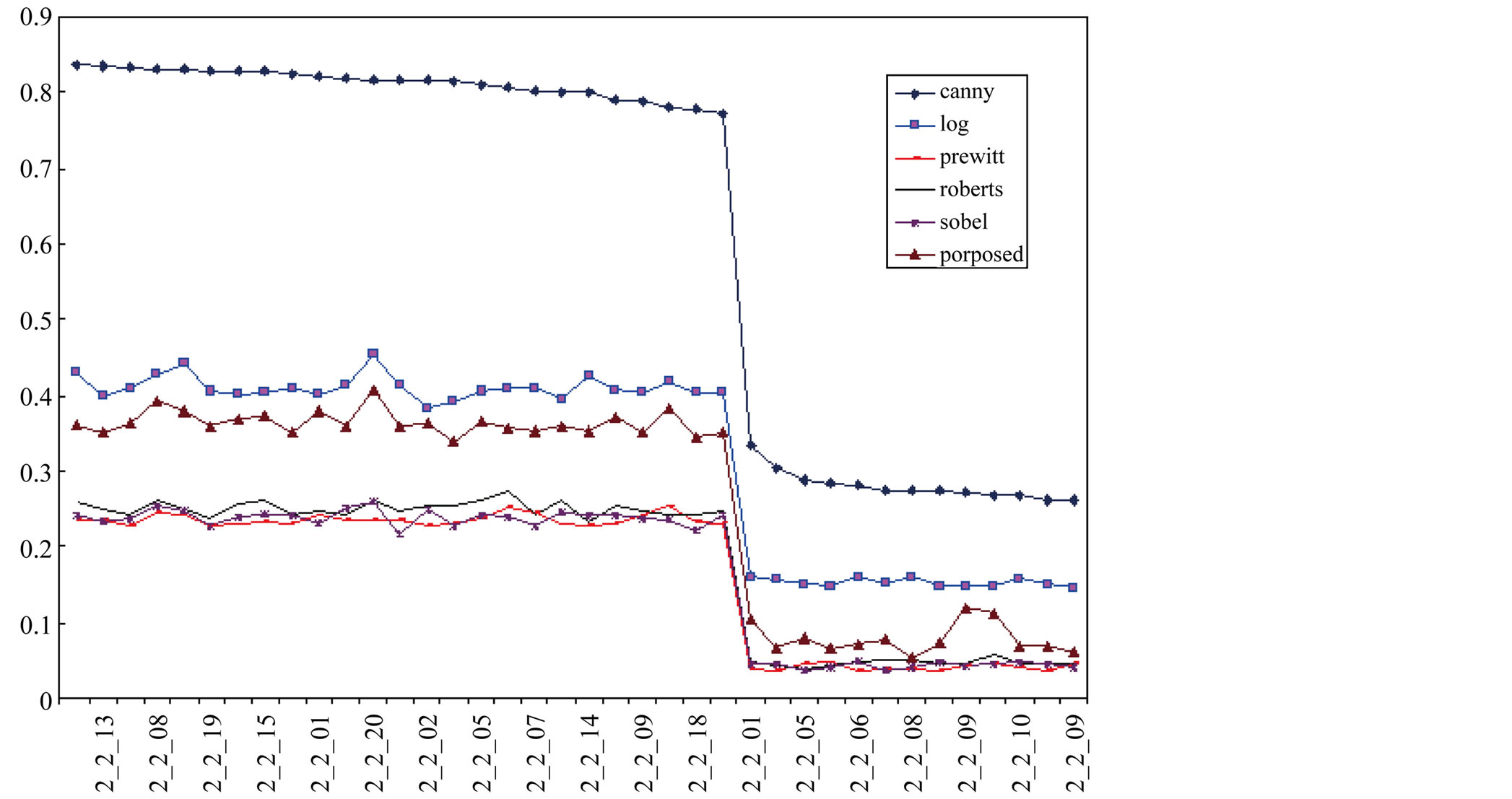
Figure 10. Comparison of run time between some classical methods and proposed method on the same datasets.
It has been observed that the proposed edge detector works effectively for different gray scale digital images as compare to the run time of classical methods. Some selected results of edge detections for these test images using the classical methods and proposed scheme are shown in Figure 11 and Table 2.
10. Conclusion
This paper shows the new algorithm based on the Havrda
& Charvat’s entropy for edge detection using split and merge technique of the histogram of grey scale image. The objective is to find the best edge representation and minimize the computation time. A set of experiments in the domain of edge detection are presented on a sample of test images, see Figure 9. An edge detection performance is compared to the previous classic methods, such as Canny, LOG, and Sobel. Analysis shows that the effect of the proposed method is better than those methods in
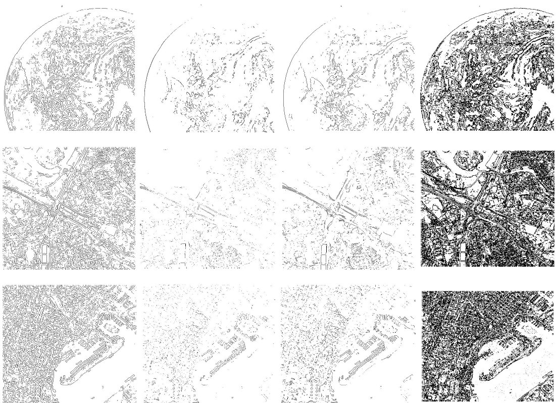
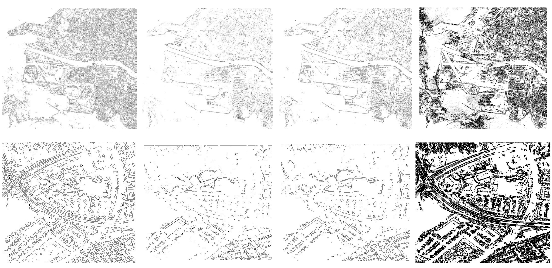
Figure 11. Edge detections of test images using the LoG method, Roberts method, Sobel method and proposed method, respectively.
execution time, and it is also considered as easy implementation. The significance of this study lies in decreasing the computation time with generate suitable quality of edge detection. It is already pointed out in the introduction
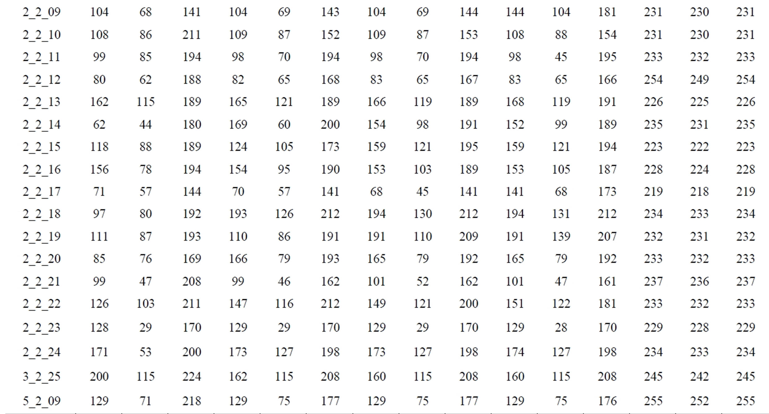
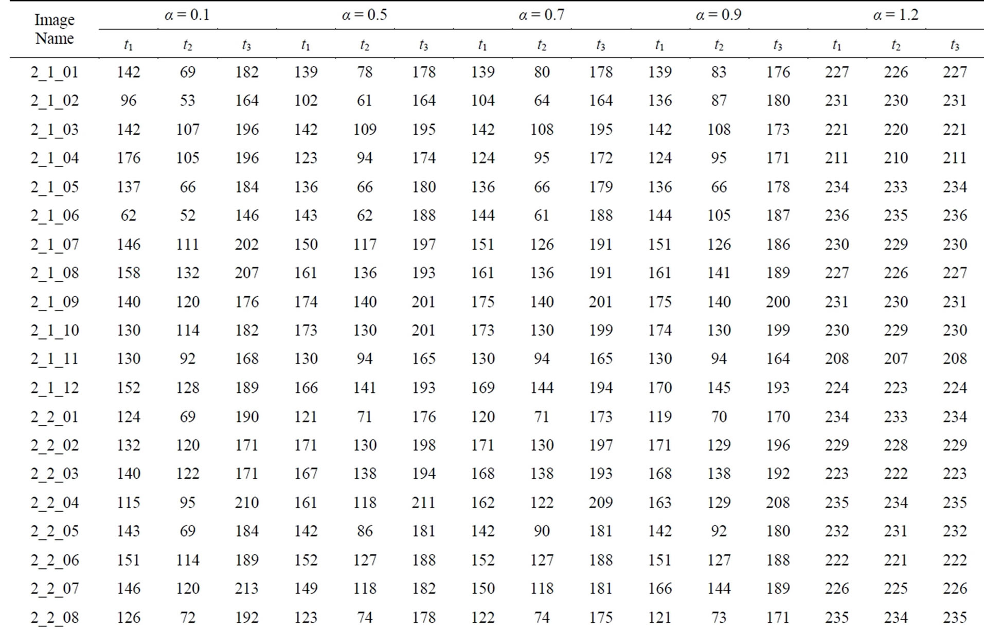
Table 2. The threshold values of tested images with different values of α.
that the traditional methods give rise to the exponential increment of computational time. Experiment results have demonstrated that the proposed scheme for edge detection can be used for different gray level digital images. Another benefit comes from easy implementation of this method. The proposed method works well as compared to the previous methods, Roberts, Prewitt, and Sobel on test samples.
REFERENCES
- S. S. Alamri, N. V. Kalyankar and S. D. Khamitkar, “Image Segmentation By Using Edge Detection,” International Journal on Computer Science and Engineering (IJCSE), Vol. 2, No. 3, 2010, pp. 804-807.
- J. Lzaro, J. L. Martn, J. Arias, A. Astarloa and C. Cuadrado, “Neuro Semantic Thresholding Using OCR Software for High Precision OCR Applications,” Image Vision Computing, Vol. 28, No. 4, 2010, pp. 571-578. http://dx.doi.org/10.1016/j.imavis.2009.09.011
- Z. Xue, D. Ming, W. Song, B. Wan and S. Jin, “Infrared Gait Recognition Based on Wavelet Transform and Support Vector Machine,” Pattern Recognition, Vol. 43, No. 8, 2010, pp. 2904-2910. http://dx.doi.org/10.1016/j.patcog.2010.03.011
- M. A. El-Sayed, “Edges Detection Based on Renyi Entropy with Split/Merge,” Computer Engineering and Intelligent Systems (CEIS), Vol. 3, No. 9, 2012, pp. 32-41.
- G. C. Anagnostopoulos, “SVM-Based Target Recognition from Synthetic Aperture Radar Images Using Target Region Outline Descriptors,” Nonlinear Analysis: Theory, Methods & Applications, Vol. 71, No. 12, 2009, pp. e2934-e2939. http://dx.doi.org/10.1016/j.na.2009.07.030
- Y.-T. Hsiao, C.-L. Chuang, Y.-L. Lu and J.-A. Jiang, “Robust Multiple Objects Tracking Using Image Segmentation and Trajectory Estimation Scheme in Video Frames,” Image Vision Computing, Vol. 24, No. 10, 2006, pp. 1123-1136. http://dx.doi.org/10.1016/j.imavis.2006.04.002
- M. T. Doelken, H. Stefan, E. Pauli, A. Stadlbauer, T. Struffert, T. Engelhorn, G. Richter, O. Ganslandt, A. Doerfler and T. Hammen, “1H-MRS Profile in MRI Positive versus MRI Negative Patients with Temporal Lobe Epilepsy,” Seizure, Vol. 17, No. 6, 2008, pp. 490-497. http://dx.doi.org/10.1016/j.seizure.2008.01.008
- S. Kresic-Juric, D. Madej and S. Fadil, “Applications of Hidden Markov Models in Bar Code Decoding,” International Journal of Pattern Recognition Letters, Vol. 27, No. 14, 2006, pp. 1665-1672.
- G. Markus, Essam A. EI-Kwae and R. K. Mansur, “Edge Detection in Medical Images Using a Genetic Algorithm,” IEEE Transactions on Medical Imaging, Vol. 17, No. 3, 1998, pp. 469-474.
- M. Wang and Y. Shuyuan, “A Hybrid Genetic Algorithm Based Edge Detection Method for SAR Image,” IEEE Proceedings of the Radar Conference’05, 9-12 May 2005, pp. 1503-506.
- A. El-Zaart, “A Novel Method for Edge Detection Using 2 Dimensional Gamma Distribution,” Journal of Computing Science, Vol. 6, No. 2, 2010, pp. 199-204.
- M. A. El-Sayed, “A New Algorithm Based Entropic Threshold for Edge Detection in Images,” International Journal of Computer Science Issues (IJCSI), Vol. 8, No. 5, 2011, pp. 71-78.
- V. Aurich and J. Weule, “Nonlinear Gaussian Filters Performing Edge Preserving Diffusion,” Proceeding of the 17th Deutsche Arbeitsgemeinschaft für Mustererkennung (DAGM) Symposium, Bielefeld, 13-15 September 1995, Springer-Verlag, pp. 538-545.
- M. Basu, “A Gaussian Derivative Model for Edge Enhancement,” Pattern Recognition, Vol. 27, No. 11, 1994, pp. 1451-1461.
- G. Deng and L. W. Cahill, “An Adaptive Gaussian Filter for Noise Reduction and Edge Detection,” Proceeding of the IEEE Nuclear Science Symposium and Medical Imaging Conference, San Francisco, 31 October-6 November 1993, IEEE Xplore Press, pp. 1615-1619.
- C. Kang and W. Wang, “A Novel Edge Detection Method Based on the Maximizing Objective Function,” Pattern Recognition, Vol. 40, No. 2, 2007, pp. 609-618.
- Q. Zhu, “Efficient Evaluations of Edge Connectivity and Width Uniformity,” Image Vision Computing, Vol. 14, No. 1, 1996, pp. 21-34.
- B. Mitra, “Gaussian Based Edge Detection Methods—A Survey,” IEEE Transactions on Systems, Man and Cybernetics, Vol. 32, No. 3, 2002, pp. 252-260.
- J. F. Canny, “A Computational Approach to Edge Detection,” IEEE Transactions on Pattern Analysis and Machine Intelligence (IEEE TPAMI), Vol. 8, No. 6, 1986, pp. 769-798.
- N. Senthilkumaran and R. Rajesh, “Edge Detection Techniques for Image Segmentation—A Survey,” Proceedings of the International Conference on Managing Next Generation Software Applications (MNGSA-08), 2008, pp. 749-760.
- K. W. Bowyer, C. Kranenburg and S. Dougherty, “Edge Detector Evaluation Using Empirical ROC Curves,” IEEE Conference on Computer Vision and Pattern Recognition (CVPR), 1999, pp. 354-359.
- M. Heath, S. Sarkar, T. Sanocki and K. W. Bowyer, “A Robust Visual Method for Assessing the Relative Performance of Edge Detection Algorithms,” IEEE Transactions on Pattern Analysis and Machine Intelligence (TPAMI), Vol. 19, No. 12, 1997, pp. 1338-1359. http://dx.doi.org/10.1109/34.643893
- M. Shin, D. Goldgof and K. W. Bowyer, “An Objective Comparison Methodology of Edge Detection Algorithms for Structure from Motion Task,” IEEE Conference on Computer Vision and Pattern Recognition (CVPR), 1998, pp. 190-195.
- R. Deriche, “Using Canny’s Criteria to Derive a Recursively Implemented Optimal Edge Detector,” International Journal of Computer Vision (IJCV), Vol. 1, No. 2, 1987, pp. 167-187. http://dx.doi.org/10.1007/BF00123164
- C. E. Shannon, “A Mathematical Theory of Communication,” Bell System Technical Journal, Vol. 27, No. 3, 1948, pp. 379-423. http://dx.doi.org/10.1002/j.1538-7305.1948.tb01338.x
- A. P. S. Pharwaha and B. Singh, “Shannon and NonShannon Measures of Entropy for Statistical Texture Feature Extraction in Digitized Mammograms,” Proceedings of the World Congress on Engineering and Computer Science (WCECS), San Francisco, Vol. II, 20-22 October 2009.
- C. Tsallis, “Possible Generalization of Boltzmann-Gibbs Statistics,” Journal of Statistical Physics, Vol. 52, No. 1-2, 1988, pp. 479-487. http://dx.doi.org/10.1007/BF01016429
- M. P. de Albuquerque, I. A. Esquef and A. R. Gesualdi Mello, “Image Thresholding Using Tsallis Entropy,” Pattern Recognition Letters, Vol. 25, No. 9, 2004, pp. 1059- 1065. http://dx.doi.org/10.1016/j.patrec.2004.03.003
- B. Singh and A. P. Singh, “Edge Detection in Gray Level Images Based on the Shannon Entropy,” Journal of Computing Science, Vol. 4, No. 3, 2008, pp. 186-191. http://dx.doi.org/10.3844/jcssp.2008.186.191