Journal of Software Engineering and Applications
Vol.5 No.7(2012), Article ID:19730,6 pages DOI:10.4236/jsea.2012.57055
A TSK-Type Recurrent Neuro-Fuzzy Systems for Fault Prognosis
![]()
1Laboratoire d’Automatique et Productique (LAP), Université de Batna, Batna, Algérie; 2Centre Universitaire Khenchela, Khenchela, Algérie.
Email: {mehdaoui.rafik, h_mouss}@yahoo.fr
Received January 26th, 2012; revised February 29th, 2012; accepted March 11th, 2012
Keywords: TSK neuro-Fuzzy Systems; Faults Diagnosis; Fault prognosis
ABSTRACT
As a result from the demanding of process safety, reliability and environmental constraints, a called of fault detection and diagnosis system become more and more important. In this article some basic aspects of TSK (Takigi Sugeno Kang) neuro-fuzzy techniques for the prognosis and diagnosis of manufacturing systems are presented. In particular, a neuro-fuzzy model that can be used for the identification and the simulation of faults prognosis models is described. The presented model is motivated by a cooperative neuro-fuzzy approach based on a vectorized recurrent neural network architecture. The neuro-fuzzy architecture maps the residuals into two classes: a one of fixed direction residuals and another one of faults belonging to rotary kiln.
1. Introduction
Failure may cause large amount of loss. Therefore, fault diagnosis and prognosis system is very important for safe operation and preventing rescue. Recent progress in the field of diagnostics of manufacturing systems (MS) drives is a result of broadly conceived basic research carried out over many years.
According to [1], there is no single method that could accommodate the entire system fault. Thus, the combination of ANN and fuzzy logic is considerably practical because it combined both of the advantages and makes the entire system more robust. ANN can operate simultaneously on qualitative and quantitative data and very useful when no mathematical model of the system is available whereas fuzzy logic has an ability to mimic the sensing, generalizing, processing, operating and learning ability of human operator [2]. In order to achieve this goal we organize this article into three parts. The first part presents principal architectures of TSK Temporal Neuro-Fuzzy systems operation and their applications. The second part is dedicated to the workshop of clinker of cement factory. Lastly, in the third part we propose a Neuro-Fuzzy system for system of production diagnosis.
2. Temporal Neuro-Fuzzy Systems
Fuzzy neural network (FNN) approach has become a powerful tool for solving real-world problems in the area of forecasting, identification, control, image recognition and others that are associated with high level of uncertainty [2].
The Neuro-fuzzy model combines, in a single framework, both numerical and symbolic knowledge about the process. Automatic linguistic rule extraction is a useful aspect of NF especially when little or no prior knowledge about the process is available [1,3]. For example, a NF model of a non-linear dynamical system can be identified from the empirical data.
This model can give us some insight about the on linearity and dynamical properties of the system.
The most common NF systems are based on two types of fuzzy models TSK [4,5] combined with NN learning algorithms. TSK models use local linear models in the consequents, which are easier to interpret and can be used for control and fault diagnosis [6]. Mamdani models use fuzzy sets as consequents and therefore give a more qualitative description. Many Neuro-fuzzy structures have been successfully applied to a wide range of applications from industrial processes to financial systems, because of the ease of rule base design, linguistic modeling, and application to complex and uncertain systems, inherent non-linear nature, learning abilities, parallel processing and fault-tolerance abilities. However, successful implementation depends heavily on prior knowledge of the system and the empirical data [7].
Neuro-fuzzy networks by intrinsic nature can handle limited number of inputs. When the system to be identified is complex and has large number of inputs, the fuzzy rule base becomes large.
NF models usually identified from empirical data are not very transparent. Transparency accounts a more meaningful description of the process i.e. less rules with appropriate membership functions. In ANFIS [2] a fixed structure with grid partition is used. Antecedent and consequent parameters are identified by a combination of least squares estimate and gradient based method, called hybrid learning rule. This method is fast and easy to implement for low dimension input spaces. It is more prone to lose the transparency and the local model accuracy because of the use of error back propagation that is a global and not locally nonlinear optimization procedure. One possible method to overcome this problem can be to find the antecedents & rules separately e.g. clustering and constrain the antecedents, and then apply optimization.
Hierarchical NF networks can be used to overcome the dimensionality problem by decomposing the system into a series of MISO and/or SISO systems called hierarchical systems [6]. The local rules use subsets of input spaces and are activated by higher level rules [7].
The criteria on which to build a NF model are based on the requirements for faults diagnosis and the system characteristics. The function of the NF model in the FDI scheme is also important i.e. Preprocessing data, Identification (Residual generation) or classification (Decision Making/Fault Isolation).
For example a NF model with high approximation capability and disturbance rejection is needed for identification so that the residuals are more accurate.
Whereas in the classification stage, a NF network with more transparency is required.
The following characteristics of NF models are important:
Approximation/Generalisation capabilities;
Transparency: Reasoning/use of prior knowledge/rules;
Training Speed/Processing speed;
Complexity;
Transformability: To be able to convert in other forms of NF models in order to provide different levels of transparency and approximation power.
Adaptive learning.
Two most important characteristics are the generalising and reasoning capabilities. Depending on the application requirement, usually a compromise is made between the above two.
In order to implement this type of Neuro-Fuzzy Systems for Fault Diagnosis and Prognosis and exploited to diagnose of dedicated production system we have to propose data-processing software NEFDIAG (NeuroFuzzy Diagnosis).
The Takagi-Sugeno type fuzzy rules are discussed in detail in Subsection A. In Subsection B, the network structure of FENN is presented.
2.1. Temporal Fuzzy Rules
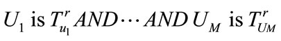
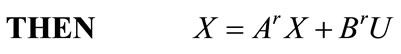
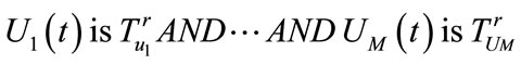
Recently, more and more attention has paid to the Takagi-Sugeno type rules [8] in studies of fuzzy neural networks. This significant inference rule provides an analytic way of analyzing the stability of fuzzy control systems. If we combine the Takagi-Sugeno controllers together with the controlled system and use state-space equations to describe the whole system [9], we can get another type of rules to describe nonlinear systems as below:
Rule r: 
where  is the inner is the inner state vector of the nonlinear system;
 is the input vector to the system, and N, M are the dimensions;
 are linguistic terms (fuzzy sets) defining the conditions for xi and uj respectively, according to Rule r;
![]() is a matrix of
is a matrix of  and
and
![]() of
of 
When considered in discrete time, such as modeling using a digital computer, we often use the discrete statespace equations instead of the continuous version. Concretely, the fuzzy rules become:
Rule r: 
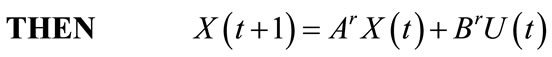
where  is the discrete sample of state vector at discrete time t. In following discussion we shall use the latter form of rules.
In both forms, the output of the system is always defined as:
 (1)
(1)
where C= (cij)Px Xis a matrix of P × N, and P is the dimension of output vector Y.
The fuzzy inference procedure is specified as below. First, we use multiplication as operation AND to get the firing strength of Rule r:
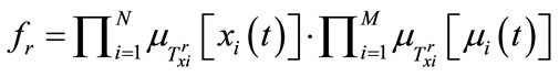 (2)
(2)
where .and
.and  are the membership functions of
 respectively? After normalization of the firing strengths, we get (assuming R is the total number of rules)
 (3)
(3)
where S is the summation of firing strengths of all the rules, and hr is the normalized firing strength of Rule r. When the defuzzification is employed, we have
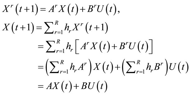 (4)
(4)
where 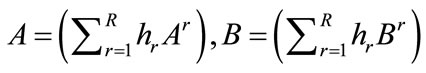
Using equation (4), the system state transient equation, we can calculate the next state of system by current state and input.
2.2. The Structure of Temporal Neuro-Fuzzy System
The main idea of this model is to combine simple feed forward fussy systems to arbitrary hierarchical models.
The structure of recurrent Neuro-fuzzy systems is presented in figure 1.
In this network, input nodes which accept the environment inputs and context nodes which copy the value of the state-space vector from layer 3 are all at layer 1 (the Input Layer). They represent the linguistic variables known as uj and xi in the fuzzy rules. Nodes at layer 2 act as the membership functions, translating the linguistic variables from layer 1 into their membership degrees. Since there may exist several terms for one linguistic variable, one node in layer 1 may have links to several nodes in layer 2, which is accordingly named as the term nodes. The number of nodes in the Rule Layer (layer 3) and the one of the fuzzy rules are the same—each node represents one fuzzy rule and calculates the firing strength of the rule using membership degrees from layer 2. The connections between layer 2 and layer 3 correspond with the antecedent of each fuzzy rule. Layer 4, as the Normalization Layer, simply does the normalization of the firing strengths. Then with the normalized firing strengths hr, rules are combined at layer 5, the Parameter Layer, where A and B become available. In the Linear System Layer, the 6th layer, current state vector X(t) and input vector U(t) are used to get the next state X(t + 1), which is also fed back to the context nodes for fuzzy inference at time (t + 1). The last layer is the Output Layer, multiplying X(t + 1) with C to get Y(t + 1) and outputting it.
Next we shall describe the feed forward procedure of TNFS by giving the detailed node functions of each layer, taking one node per layer as example. We shall use notations like  to denote the ith input to the node in layer k, and o[k] the output of the node in layer k. Another issue to mention here is the initial values of the context
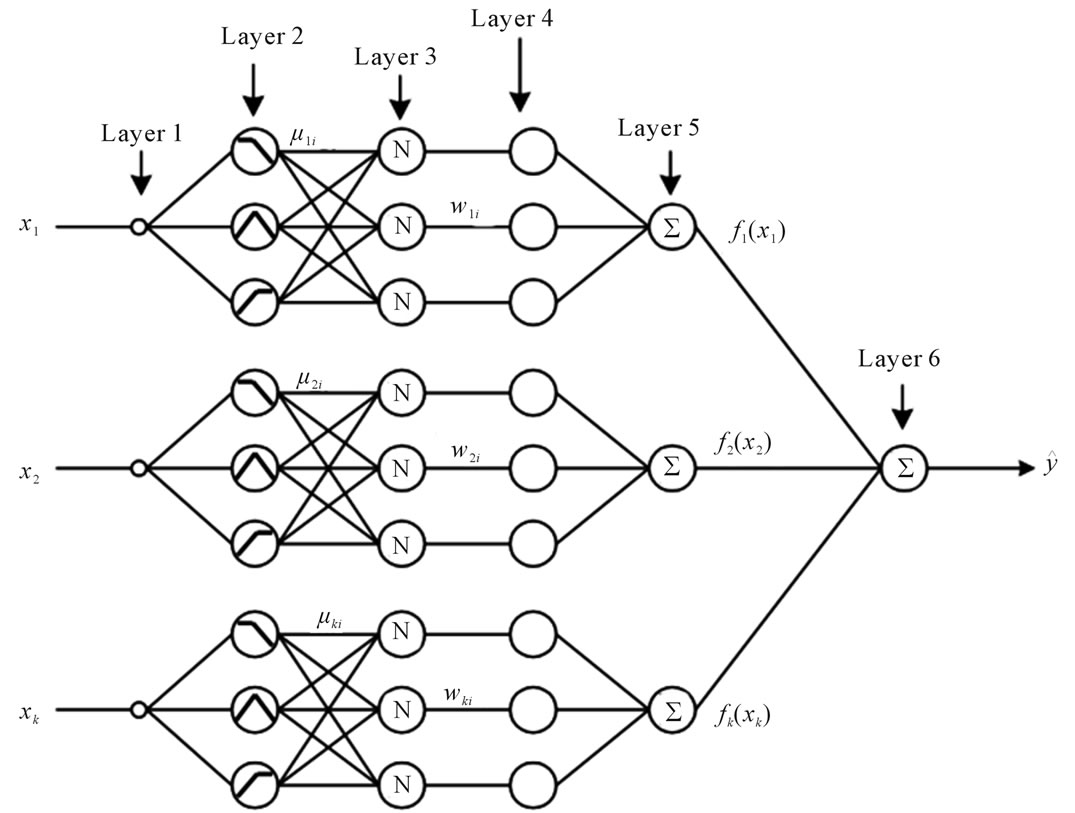
Figure 1. The structure of a simple TNFS.
nodes. Since TNFS is a recurrent network, the initial values are essential to the temporal output of the network. Usually they are preset to 0, as zero-state, but non-zero initial state is also needed for some particular case.
Layer 1. There is only one input to each node at layer 2. The Gaussian function is adopted here as the membership function:
 (5)
(5)
where cr and sr give the center (mean) and width (variation) of the corresponding u[1] linguistic term of input u[2] in Rule r.
Layer 2. This layer has several nodes, one for figuring matrix A and the other for B. Though we can use many nodes to represent the components of A and B separately, it is more convenient to use matrices. So with a little specialty, its weights of links from layer 4 are matrices Ar (to node for A) and Br (to node for B). It is also fully connected with the previous layer. The functions of nodes for A and B are respectively.
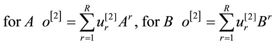 (6)
(6)
Layer 3. The Linear System Layer has only one node, which has all the outputs of layer 1 and layer 2 connected to it as inputs. Using matrix form of inputs and output, we have
3. Prognostics Process
The first step in building a prognostics system, as published in the ISO standard, is the identification of the set of failure modes (FM), their influence factors on each other and the detection measures (descriptors) that allow to track the evolution of the degradation. The international standard IEC 60812 [10] has presented a procedure named “Procedure for failure mode and effects analysis (FMECA)”, which helps the identification of all the failure modes for a specific system, by the analysis of its subsystem s and components. Also, the FMECA method classifies the FMs using risk priority numbers (RPN) that are calculated with three failure mode parameters: occurrence (Occ), detection (Det) and severity (Sev). So, the FMECA [11] allows the definition of the appropriate detection method and measures to be used in the diagnostics as well as in the prognostics of the failure modes.
The network structure is build in three steps:
Step 1. The determination of fuzzy subsets for every input variable. The initial values of the centres and variances characterising the membership functions of the first layer down, can be arbitrarily established (equidistant on the domain of definition of the linguistic variable) or applying a clustering algorithm of the type Fuzzy C-Means.
Step 2. Obtain the minimal dimension of the rule base.
The extraction of most significant rule that determines the number of the nodes in the second layer.
Step 3. Optimization of the parameters of rules determined at Step 2. The objective is to alternate the parameter values (c,w) of the network in order to improve the rule base minimizing the quadratic criteria of performance,
4. Experimental Results
To test the quality of the model, several actions were generated, and fixed goals were defined. The goals were defined in a way that the results were understood without ambiguity by human knowledge, the figure 2 illustrate the fuzzy base rules with 3 parametres to classify the defaults modes In order to illustrate the learning effect of the proposed immune based FNN (IM-FNN), we use One of the most important types of systems present in the process industry is workshop of SCIMAT clinker. A fault in a workshop of SCIMAT clinker may lead to a halt in production for long periods of time. Apart from these economic considerations faults may also have security implications. A fault in an actuator may endanger human lives, as in the case of a fault in an elevator’s emergency brakes or in the stems position control system of a nuclear power plant [9,12]. The design and performance testing of fault diagnosis systems for industrial process often requires a simulation model since the actual system is not available to generate normal and faulty operational.
In figure 3 the detection of fault mode in the rotary kiln is observed with the classification after training the neuro-fuzzy system.
data needed for design and testing, due to the economic and security reasons that they would imply. Accord-
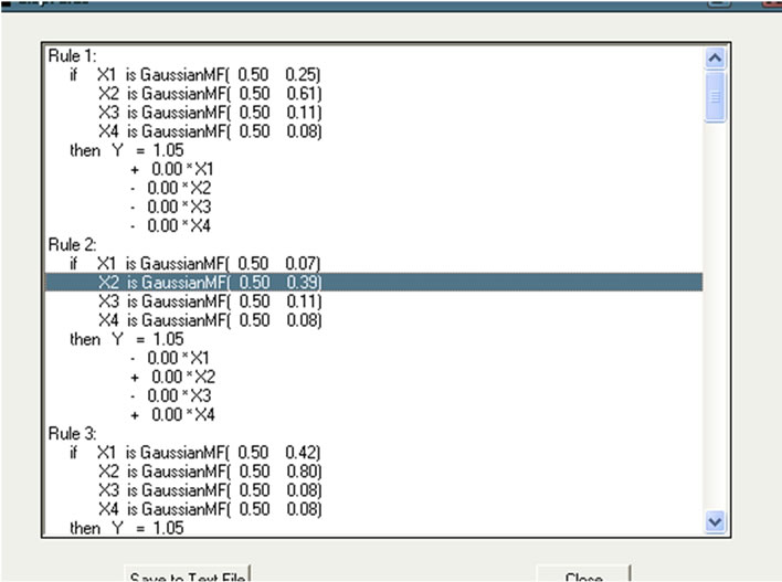
Figure 2. the generated rules base.

Figure 3. Detection of fault mode.
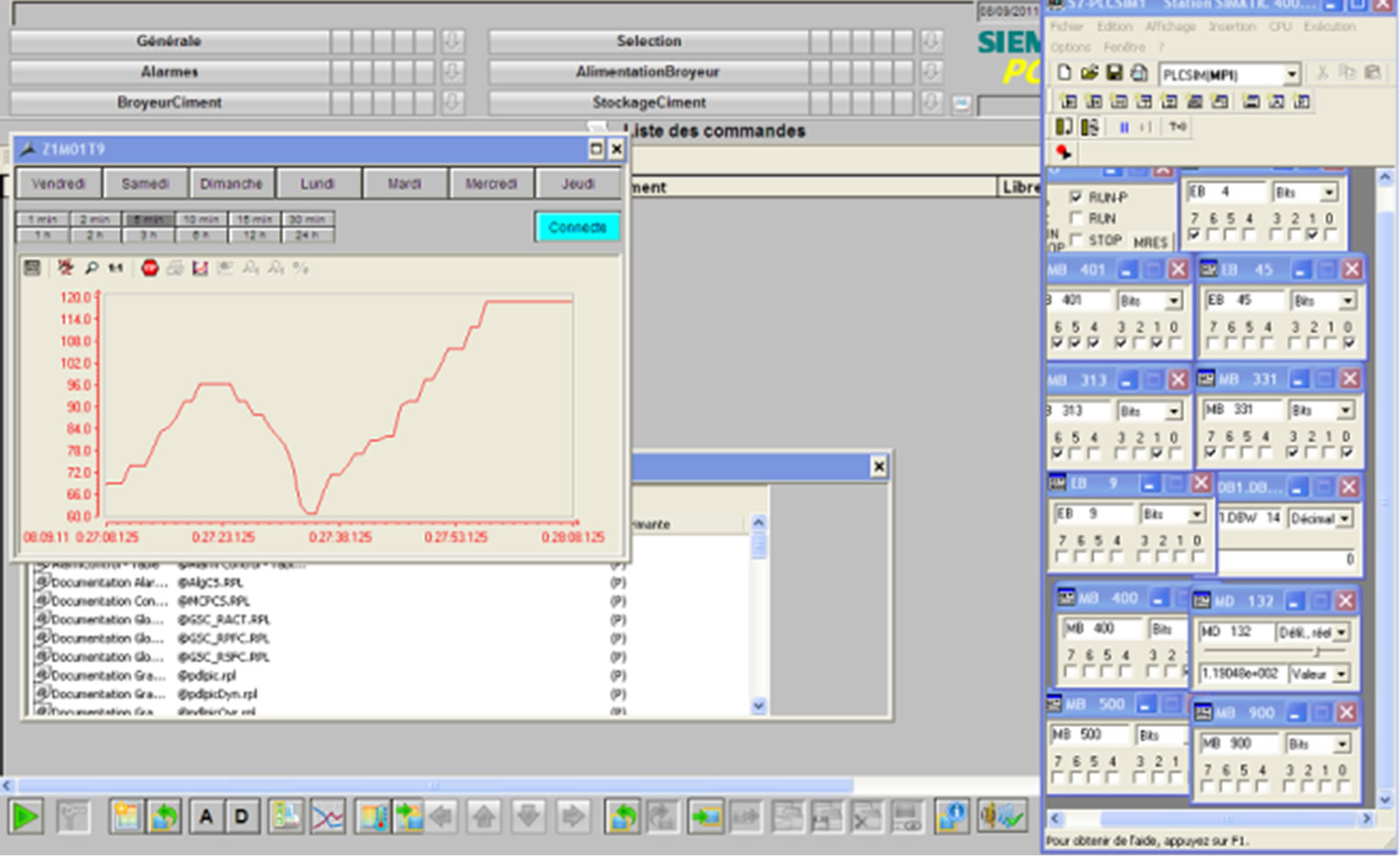
Figure 4. The failure mode of rotary kiln.
ing to this figure 4 we can say the prediction of a faults is a complex problem and need the correction of inverse problem.
5. Conclusion
The successful of implementing neuron-fuzzy is heavily depends on prior knowledge of the system and the training data. In the intrinsic nature, the neuro-fuzzy only can handle a limited number of inputs and can usually be identified in a not very transparent way from the empirical data [2]. The transparency is the determination of the process with a less amount of fuzzy rules with appropriate membership function. For the complex system, a large architecture is needed to represent a model.
REFERENCES
- R. J. Patton, P. M. Frank and R. N. Clark, “Issues of Fault Diagnosis for Dynamic Systems,” Springer, London, 2000.
- L. Marinai, “Gas Path Diagnostics and Prognostics for Aero-Engines Using Fuzzy Logic and Time Series Analysis,” Ph.D. Thesis, School of Engineering, Canfield University, Canfield, 2004.
- J. M. Koscielny and M. Syfert, “Fuzzy Logic Applications to Diagnostics of Industrial Processes,” Preprints of the 5th IFAC Symposium on Fault Detection, Supervision and Safety for Technical Processes, Washington, 9-11 June 2003, pp. 771-776.
- C.-F. Juang, “A TSK-Type Recurrent Fuzzy Network for Dynamic Systems Processing by Neural Network and Genetic Algorithms,” IEEE Transactions on Fuzzy Systems, Vol. 10, No. 2, 2002, pp. 155-170. doi:10.1109/91.995118
- C. D. Bocaniala and J. Sa da Costa, “Tuning the Parameters of a Fuzzy Classifier for Fault Diagnosis. HillClimbing vs Genetic Algorithms,” Proceedings of the 6th Portuguese Conference on Automatic Control, Faro, 7-9 June 2004, pp. 349-354.
- J. He, “Neuro-Fuzzy Based Fault Diagnosisf or Nonlinear Processes,” Ph.D. Thesis, The University of New Brunswick, New Brunswick, 2006.
- F. J. Uppal and R. J Patton, “Fault Diagnosis of an Electro-pneumatic Valve Actuator Using Neural Networks with Fuzzy Capabilities,” 2002.
- C. D. Bocaniala, J. Sa da Costa and V. Palade, “A Novel Fuzzy Classification Solution for Fault Diagnosis,” International Journal of Fuzzy and Intelligent Systems, Vol. 15, No. 3-4, 2004, pp. 195-206.
- K. B. Ariffin, “On Neuro-Fuzzy Applications for Automatic Control, Supervision, and Fault Diagnosis for Water Treatment Plant,” Ph.D. Thesis, Faculty of Electrical Engineering Universiti, Teknologi, 2007.
- D. Henry, X. Olive and E. Bornschlegl, “A Model-Based Solution for Fault Diagnosis of Thruster Faults: Application to the Rendezvous Phase of the Mars Sample Return Mission,” European Conference for Aero-Space Sciences, St. Petersburg, 4-8 July 2011.
- F. Xi, Q. Sun and G. Krishnappa, “Bearing Diagnostics Based on Pattern Recognition of Statistical Parameters. Journal of Vibration and Control, Vol. 6, No. 3, 2000, pp. 375-392. doi:10.1177/107754630000600303
- J. Biteus, “Distributed Diagnosisand Simulation Based Residualgenerators,” Ph.D. Thesis, Vehicular SystemsDepartment of Electrical Engineering, Linkopings Universitet, Linkoping, 2005.