Intelligent Information Management
Vol.6 No.2(2014), Article ID:44319,26 pages DOI:10.4236/iim.2014.62008
An Agent-Based Assessment of Land Use and Ecosystem Changes in Traditional Agricultural Landscape of Portugal
Lilibeth A. Acosta1,2, Mark D. A. Rounsevell3, Martha Bakker4, Ann Van Doorn5, Montserrat Gómez-Delgado6, Marc Delgado7
1Potsdam Institute for Climate Impact Research, Potsdam, Germany
2School of Environmental Science and Management, University of the Philippines Los Baños, Los Baños, Philippines
3School of GeoSciences, University of Edinburgh, Edinburgh, UK
4Land Use Planning Group, Wageningen University and Research Centre, Wageningen, The Netherlands
5Alterra, Environmental Sciences Group, Wageningen, The Netherlands
6Departamento de Geología, Geografía y Medio Ambiente, Unidad docente de Geografía, Universidad de Alcalá, Alcalá de Henares, España
7Department of Geography, Faculty of Sciences, Vrije Universiteit Brussel, Brussel, Belgium
Email: lilibeth@pik-potsdam.de, mark.rounsevell@ed.ac.uk, Martha.Bakker@wur.nl, anne.vandoorn@wur.nl, montserrat.gomez@uah.es, mdelgado@vub.ac.be
Copyright © 2014 by authors and Scientific Research Publishing Inc.
This work is licensed under the Creative Commons Attribution International License (CC BY).
http://creativecommons.org/licenses/by/4.0/


Received 10 February 2014; revised 4 March 2014; accepted 24 March 2014
ABSTRACT
This paper presents an assessment of land use changes and their impacts on the ecosystem in the Montado, a traditional agricultural landscape of Portugal in response to global environmental change. The assessment uses an agentbased model (ABM) of the adaptive decisions of farmers to simulate the influence on future land use patterns of socio-economic attributes such as social relationships and farmer reliance on subsidies and biophysical constraints. The application and development of the ABM are supported empirically using three categories of input data: 1) farmer types based on a cluster analysis of socio-economic attributes; 2) agricultural suitability based on regression analysis of historical land use maps and biophysical attributes; and 3) future trends in the economic and climatic environments based on the A1fi scenario of the Intergovernmental Panel on Climate Change. Model sensitivity and uncertainty analyses are carried out prior to the scenario analysis in order to verify the absence of systematic errors in the model structure. The results of the scenario analysis show that the area of Montado declines significantly by 2050, but it remains the dominant land use in the case study area, indicating some resilience to change. An important policy challenge arising from this assessment is how to encourage next generation of innovative farmers to conserve this traditional landscape for social and ecological values.
Keywords:Abandonment; Agent-Based Model; Cluster Analysis; Ecosystem and Biodiversity; Land Use Change; Logistic Regression; Portugal; Scenario Analysis; Traditional Agricultural Landscape

1. Introduction
Traditional, low intensity agricultural areas in Europe are increasingly appreciated by society for their biodiversity, landscape value and cultural functions. This is reflected in the shift in focus of the Common Agricultural Policy (CAP) from the dominant paradigm of agricultural price/income support before the mid 1990s to agrienvironmental measures (AEM) from the early 2000s. The Alentejo region of Portugal is known for a traditional agricultural landscape known as “Montado”. Montado is a multifunctional silvo-pastoral system combining holm or cork oak with extensive livestock grazing (e.g. sheep, goats, cattle, pig) and/or cereal cultivation. Of the 800,000 hectares of Montado in Portugal, about 90 percent is located in the Alentejo [1] [2] . The mosaic of montado habitats supports a rich diversity of animals [3] . Nutrient cycles are maintained by the manure of animals that feed on acorns, shrubs and grasses under the trees and infiltration of precipitation in the soil is promoted through careful tree management and controlled grazing [4] . The management of Montado in the past has also included the conservation of oak trees, either by natural regeneration or by artificial seeding or planting to maintain cork production [5] . Montado is a complex, socio-ecological system that depends on human practices and management for its conservation and continuation [6] [7] providing an example of where human and natural dynamics are integrated in a reciprocal and complementary relationship [7] . Montado has survived throughout the 20th century in spite of the large economic changes experienced in Portugal in the second half of the century that changed the management practices and resources used by Montado farmers, but not the area of open oak grasslands [3] . As one of the poorest regions in the EU, the Alentejo receives support from the European Union (EU) both through AEM subsidies and less favoured area (LFA) payments and these subsidies have been crucial in conserving the Montado landscape during difficult economic times.
The complexity of the Montado system arises from production activities sharing the same growing space in a landscape with site-specific soil, climatic and topographical characteristics [2] . An important characteristic of these landscapes is their high spatial and temporal variation, with patch patterns representing direct responses to varying habitat conditions and cycles of disturbance and recovery [1] . Similar to other countries within the Mediterranean basin, Portugal is characterised by large climatic variability and unpredictability (especially rainfall), which makes the diversification of agricultural production an important adaptation strategy [6] . In the Montado landscape, the occurrence of multiple land use activities within the same geographic space requires careful management to support a sustainable equilibrium [2] , mimicking natural ecosystem processes [7] -[9]. Thus, the diverse land use mosaics that characterise the Montado landscape arise from continuous social and economic adaptation to the constraints imposed by a harsh natural environment. Insight into human adaptation is important, therefore, in understanding forms of resource exploitation and the functioning of these complex land use systems [6] . Building models of these systems can assist in understanding how they function, but also support explorations of how they might respond to environmental and socio-economic change drivers in the future. Models used for this purpose need, however, to be capable of representing the effects not only of economic, environmental and policy drivers, but also the social dimensions of the decision-making and adaptation processes.
The concept of multi-agent systems, which originated in the computer sciences in the 1970s (through artificial intelligence research), has gained popularity more recently in the social sciences, for example, in linking human and natural systems across spatial and temporal scales. Land use change models based on multi-agent systems are designed to integrate human decision processes into a location-specific context in order to explain patterns of land use or settlement and test understanding of land use functions [10] . Many of these studies have been theoretical and agent-based models (ABM) of agricultural land use in particular are often not supported by empirical data [11] . The empirical application of ABM in contemporary social sciences is, however, challenging [12] . In spite of this, more recent studies have used empirical data to capture land use decision processes as they occur in practice [e.g. [13] -[19]]. These studies seek to take advantage of the key strengths of ABM in capturing the heterogeneity of agent profiles, the dynamics of their interactions and their behaviour in response to the geography of physical space. These attributes of ABM are especially useful when exploring land use change futures, where farmer decisions are influenced not only by changes in the economic and climatic environments, but also by their social and cultural values.
This paper presents an ABM of a socio-ecological system representing the Montado in the Alentejo that is informed by empirical data from social survey about the behaviour and heterogeneity of farmers. The purpose of the model is to simulate changes in land use and thus ecosystem arising from the adaptive decisions of farmers in response to changes in key drivers, i.e. economics, climate change and social change. In particular, the model is used to explore the influence on future land use patterns of socio-economic attributes including social behaviour and farmer reliance on subsidies. The study is located in the village of Amendoeira da Serra in the Alentejo region of Portugal. Whilst ABM is increasingly applied to assess land use changes, to our knowledge, no similar agent-based studies have been so far conducted in this region. Section 2 describes the case study area. Section 3 presents the methods for the land use change simulations using the ABM and Section 4 discusses the results of the simulation experiments. The conclusions are presented in Section 5.
2. The Case Study Area
The agricultural village of Amendoeira da Serra is located in the municipality of Mertola in the Alentejo region at 37˚40'N, 7˚47'E in southeast Portugal (Figure 1). The Alentejo region has a typical Mediterranean climate, characterised by hot summers with up to 5 dry months and irregular distribution of rainfall over the wetter parts of the year. It has in the past experienced frequent periods of drought, accompanied by regular wildfires and intensive flooding. The municipality is situated on the borders of the Guadiana River and has a topography of gently sloping, hilly land with altitudes ranging from 200 to 250 m above sea level. The river is the main source of surface water in the Alentejo region and in the past water supply has been affected by serious droughts [20] . More than 50 percent of the area is characterised by bedrock or very thin soils that have little agricultural potential. Due to these extreme biophysical conditions and the limited accessibility of the region, agriculture is extensive. Mertola is one of the most sparsely populated regions of Europe accounting for only about 5 percent of the population of the Alentejo and with a population density of 6.6 inhabitants per km2. The municipality continues to suffer from population decline, which was 11 percent between 1991 and 2001, resulting from an increase in alternative employment opportunities in urban areas following Portugal’s entry into the European Union (EU).
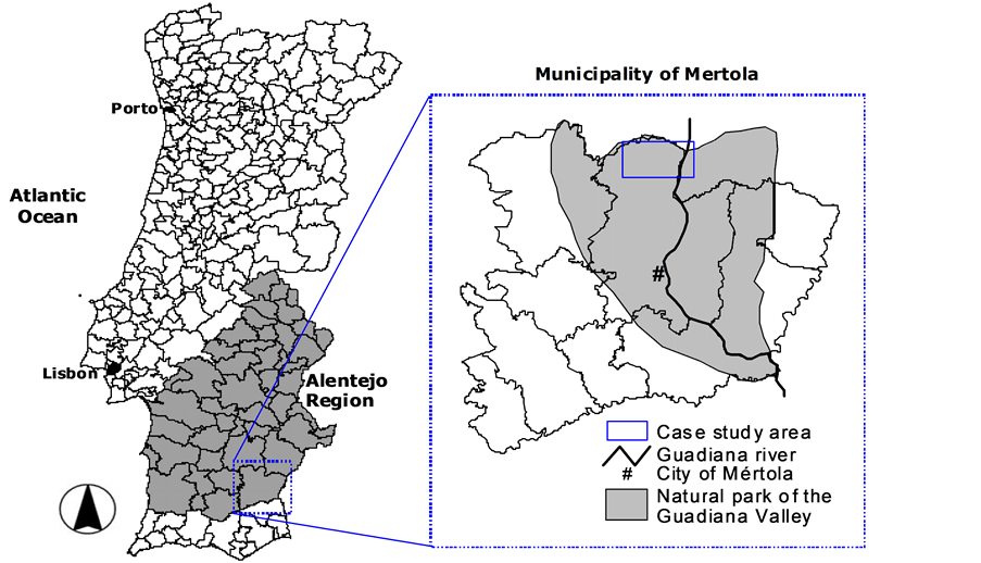
Figure 1. Location of the case study area.
The case study covers an area of 44 square km around the village of Amendoeira da Serra (Figure 1). Table 1 presents a summary of the socio-economic attributes of the farmers in the area derived from a semi-structured, social survey. The farmer population is relatively old with an average age of 59 years. The area is characterised by a low level of education with most farmers having less than 5 years of education. The average farm size is 124 hectares, but the size of individual farms is variable with rural landowners normally owning less than the urban (absent) landowners. Only 21 percent of the farmers live outside the municipality, mostly in urban areas. About 39 percent, in particular farmers with large farms employ agricultural workers. More than half of the interviewed farmers inherited their land and have been in farming for more than 10 years. The interviews indicated that farmers seldom discuss their farming activities and decisions with one another. Farmer organisations are an important source of information about farm management for some farmers. Montado remains an important farm management strategy, but the area is also characterised by forest and shrub lands and a little arable land. Agri-environmental and forestation policies resulted in the widespread conversion of arable land to forest plantation (e.g. pine, eucalyptus) with little thought for the environmental consequences of these management practices [21] . Almost 70 percent of the farmers have shrub lands, which are mostly kept for hunting purposes with hunting mostly established on large farms owned by non-resident landowners [22] . Except for shrub lands, all major land uses in the area receive subsidises. Thus the diverse land use pattern is influenced by the availability of subsidies as well as biophysical constraints [see e.g. [5] -[7] [23] .
3. Methods
The methods for the empirical application of the ABM are presented here following the ODD (Overview, Design concepts, Details) protocol [24] [25] . The ODD protocol has standardised guidelines to describe individual-based and agent-based models that aim to make model descriptions more understandable, complete and comparable. The following sections provide, therefore, information on the ABM’s 1) purpose; 2) entities, state variables, and scales; 3) process overview and scheduling; 4), design concepts; 5) input data; 6) initialisations and 7) submodels.

Table 1. Socio-economic characteristics of farmers in the case study area.
Source: Interviews in the case study area 2004.
3.1. Purpose
The model was developed within the VulnerabIlity of Ecosystem Services to Land Use Change in Traditional Agricultural Landscapes (VISTA) Project. The purpose of the model was to understand the influence of global environmental change drivers and land manager decisions on the future of the Montado in Portugal as an example of a traditional agricultural landscape. The aim being to generate future projections of land use change from 2000 to 2050 that account for global economic and climatic changes. Future projections were based on the storylines of the Intergovernmental Panel on climate change (IPCC) Special Report on Emissions Scenarios (SRES) with a focus on an application of the model using the A1fi storyline. The A1fi storyline represents a globalised, market-orientated world that has a fossil fuel intensive energy mix.
3.2. Entities, State Variables and Scales
The model consists of five entities including individual farmers, typology groups, grid cells, farm parcels, and environment. The individual farmers and grid cells are low-level entities, and the typology groups and farm parcels represent their collective entities, respectively.
The state variables that influence the decisions of individual farmers include age, education, profession, residence, time spent on farm (i.e. fullor part-time), years in the farm business and availability of a successor. Data describing these attributes were collected from field interviews. The model runs annually, with farmers becoming older through time until they reach the age of 65 after which they retire and a family member takes over if there is a successor.
The typology groups describe the collective characteristics of individual farmers and were identified through cluster analysis of their socio-economic attributes (see Section 3.5). Four types were considered in the model: innovative, active, absentee, and retiree, with farmers in each type making land use decisions in distinct ways. Farmers are also allowed to change type. All farmers who retire at the age of 65 become the retiree type. Except for age the family successor adopts the individual and collective characteristics of his predecessor. Thus, the former adopts the previous type (e.g. innovative, active, or absentee) of the latter before he becomes a retiree. Farmers with a high level of education and who accumulate land over time become innovative.
Grid cells at a resolution of 20 m were characterised with an agricultural suitability attribute (see Section 3.5). A farm parcel is a collection of grid cells, which represent the farmland owned by individual farmers. Information about farm ownership was collected from cadastral archives and interviews with farmers and agricultural administrators. The land use decisions of individual farmers are made on the basis of the suitability levels of each grid cell so that only parts of the farm parcel that are suitable are converted into a new land use.
The environment, which influences how individual farmers make decisions, is defined by economic and climatic parameters. The economic parameters include costs of production such as fertilizers, pesticides, labour, and land (i.e. rental price) as well as market prices and government subsidies. The climatic parameters are represented by the effects of temperature and atmospheric CO2 concentrations on yields. The values of the parameters change on an annual basis during the simulation years from 2000 to 2050 (see Section 3.5).
3.3. Process Overview and Scheduling
The model was constructed using the NetLogo software [26] , which has several advantages for this type of application [27] [28] : 1) it is appropriate for modelling mobile agents acting concurrently across a grid space with behaviour dominated by local interactions over short time periods; 2) it has a powerful programming language that is easy to use due to a built-in graphical interface and extensive documentation; and 3) it is an open-source software with a large community of users interacting through the internet. NetLogo recognises three groups of variables known as turtles, patches and globals. In the model presented here, the individual farmer types are the turtles, the grid cells with corresponding agricultural suitability are defined as the patches and the environment, comprising the economic and climatic parameters, are the globals. In technical terms, the globals provide the information that is accessible to both patches and turtles, which analytically means defining the current and future economic and climatic environments of both patches and turtles. Values are assigned to global variables such as prices, subsidies and yields for the base year 2000, and these are perturbed through time for an economic and climatic scenario based on the IPCC SRES A1fi storyline. Thus, the globals, as exogenous variables, are responsible for the temporal dynamics in the model. The patches create the spatial characteristics of the model as represented in the maps of agricultural suitability, which take into account the biophysical properties of the farms. Physical change processes (e.g. soil degradation) are not represented through the patches. A previous analysis for the same study area suggested that correlations between socio-economic characteristics and biophysical characteristics are largely absent [29] . For this reason, it is not essential to take into account physical change processes that will only add to the complexity of the model. Whilst globals are dynamic in time and patches vary in space, turtles are adaptive to these changes over time and across space.
The adaptive decisions of the farmers depend on a number of rules and these rules were derived from a qualitative analysis of the interview results. For example, 1) farmers remember their past income and change land use if their income declines over the last three years; 2) farmers with higher education, but with decreasing farm income, look for employment outside of agriculture; 3) farmers who reach retirement abandon their land if they do not have a successor; and 4) farmers change land use only if their land is suitable for another crop. Underpinning these rules is the assumption that farmers have cognitive abilities that enable them to process information and that these abilities are influenced by the farmers’ attributes. Cognition is an important component of the adaptation of individuals to changes in their environment ([30] [31] ). Three spatial allocation rules (i.e. adaptive strategies) for farmer land use decisions are included in the model: 1) maximization; 2) repetition, and 3) imitation. The adaptive decisions in response to changes in the environment of each farmer type are presented in the decision tree (Figure 2), which provides a framework for the empirical application of the ABM. This framework combines information from the descriptive analysis of the typology groups and the assumptions underpinning the A1fi scenario.
Within the application framework, innovative farmers with large farms and better education levels are more responsive to economic opportunities or risks. The model assumes that the main strategy of the innovative farmers in response to changes in their environment is maximization. To maximize income, the innovative farmers regularly monitor their income to identify the opportunities offered from cultivating alternative crops. Moreover, if their income drops below the minimum income level in the last three consecutive years, they look for alternative crops, but always by appraising the suitability of their land for these crops. If agricultural suitability is low, they continue to cultivate the same crops (i.e. repetition). In the model, the suitability check is carried out using agricultural suitability maps (see Section 3.5). Although active farmers are not as explorative as innovative farmers, they are assumed to be able to receive and respond to available information. In the A1fi scenario, globalisation is assumed to enhance the transfer of information, for example, through the media. However, the rate of transfer of information to the active farmers is assumed to be slower than for the innovative farmers. Access to information enables some active farmers to carry out maximization, particularly those with larger farms. However, if their land is not suitable for conversion to other crops, then active farmers also engage in repetition. Regardless of farm size, active farmers with a higher level of education and whose farms are not economically viable abandon their land. Land abandonment results from low agricultural profitability and availability of alternative non-farming activities in a fast growing global economy. The retiree farmers, who retire without a successor, also abandon their land if there are no land buyers. The absentee farmers do not abandon their land even if their farm income becomes too low since they are assumed to retain their land holdings for personal reasons or future investment purposes. Because absentee farmers prefer to maintain the existing land use, they engage in repetition. However, they also imitate the neighbouring innovative farmers, who change their land use for economic reasons. It is assumed that absentee farmers visit their farm once a year allowing them to engage in imitation.
3.4. Design Concepts
Basic principles: The adaptive strategies (i.e. maximization, repetition, imitation) are based on the results of the farmer interviews as well as the economic, social and behavioural theories described in Jager et al. [32] . Whilst the maximization strategy is guided by economic decisions, imitation is influenced by the social relationships between farmers.
Emergence: The model explores the relationship between two related emergent phenomena—land abandonment and land use pattern. These emerge from the autonomous decisions of individual farmers in response to the changes in the socio-economic environment and are dependent on the adaptive strategies inherent in the farmer typology (i.e. innovative, active, absentee, and retiree). The farmer type is not fixed and can change depending on age, farm size and the accumulation of land properties.
Adaptation and objectives: adaptation is represented through the decision making strategies of individual farmers. The main objective in adapting is to prevent income loss resulting from perturbations in the economic and
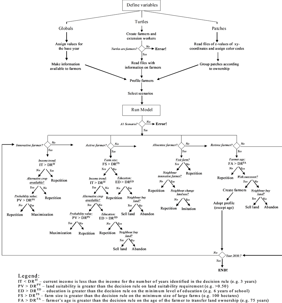
Figure 2. Agent decision tree for the agent-based model.
climatic environment and this is achieved through income maximization, as well as through social relationships, in particular imitation of neighbours.
Learning and prediction: Farmers engaging in maximization monitor farm income over the last three years and look for alternative land uses if the income declines consistently. This is a learning process from which farmers make predictions about the future. Prediction is however implicit in that farmers assume that the declining income trend will continue in the following years. Farmers who imitate are also assumed to learn from neighbours or other farmers in the area and thus implicitly predict that following other farmers decisions will bring them a higher income.
Sensing: The individual farmers are assumed to have access to current information on production costs, market prices and government subsidies, so they are able to compute revenues from, and make decisions about, alternative land uses. They have information on the impacts of technology, but not about future climatic parameters and their effects on crop yields. For income maximization, farmers base their decisions about crop yields on previous years. They know the location of their farm parcels and the agricultural suitability of each grid cell. They also know the farming activities of their neighbours.
Interaction: Interaction is assumed when innovative farmers buy farm parcels from retiree farmers who do not have successors and from active farmers who migrate to seek non-agricultural employment. Absentee farmers interact with neighbouring farmers by imitating their land use decisions. The analysis of adjacent grid cells represents farmers exchanging information.
Stochasticity: Stochasticity is kept to a minimum in the model in order to replicate as closely as possible the situation observed in reality. The values of the input variables and parameters were collected from interviews and generated from statistical analysis of actual data, except for the age of the successors, which was randomly derived due to lack of data.
Collectives: Typology groups are collectives of individual farmers and farm parcels are collectives of grid cells.
Observation: Observations include the graphical display of annual changes in land use pattern and trends, farm parcel size, proportion of types and mean income from different farming activities.
3.5. Input Data
The model requires three categories of input data to assess the effects of economic and climatic change on land use decisions and patterns: 1) farmers and farm types; 2) land use and agricultural suitability; and 3) future trends in the economic and climatic environments. The farmer typology classifies different farmer types according to the socio-economic attributes that influence land use decisions. The types were identified using cluster analysis of socio-economic data collected from interviews with farmers. Similar analyses were carried out by van Doorn and Bakker [33] . Agricultural suitability is derived statistically from the biophysical attributes that constrain land use decisions. Suitability is represented as a spatially-explicit probability map that was generated from a regression analysis of land use with soil attributes, slope, elevation and distance to rivers [see also [34] ]. Future trends in the economic and climatic baselines were based on the A1fi scenario for the period 2000 to 2050. The methods for generating the scenario parameters were drawn from other studies by interpreting the IPCC SRES storylines [35] for Europe [36] -[38].
Farmers and farmer types: Face-to-face interviews (based on a semi-structured questionnaire) were conducted in the spring/summer of 2004 to collect information about the socio-economic attributes, agricultural practices and farm management decisions of the case study farmers. The interviews covered 28 farmers, who represent more than 90 percent of the total number of farmers in Amendoeira da Serra. Information from the interviews as well as cadastral archives and regional agricultural administration data were used to map the structure of farmer properties (Figure 3). This map is used in the model to represent the farmers’ land ownership and location. The farmer typology is important in generalising agent behaviour with types being identified from a cluster analysis of the farmers’ socio-economic attributes. This method is increasingly used in land use studies to group agents based on their attributes [e.g. [7] [14] [39] ]. The socio-economic variables that were used in the cluster analysis are given in Table1 The cluster analysis followed the two-step approach described in Hair et al. [40] , which combines both hierarchical and non-hierarchical clustering procedures to arrive at a cluster solution. This approach is appropriate here since compared with other cluster approaches it can efficiently combine both categorical and continuous dataset [41] .
Four clusters were identified from the cluster analysis (see Annex A for the method and results of the cluster analysis). Matrix scoring was applied on these clusters to identify the farm types. The types define the farmers’ attributes for each of these clusters and are characterised as innovative, active, absentee, and retiree (Table 2). Innovative farmers are fewer in number, but they own the largest properties and have the highest level of education. These farmers have diversified activities including, amongst others, livestock breeding, hunting, forestry and nature protection. Innovative farmers have the willingness to explore new farming techniques through personal contacts both within (not necessarily in the case study area) and outside of Portugal. These farmers seldom exchange ideas about farming management with one another (Section 2), which reflects to some extent the poor social network in Amendoeira da Serra. Thus it is assumed that the knowledge of innovative farmers isnot easily transferred to other farmer types. Innovative farmers have only an indirect influence on other farmers through imitation within the neighbourhood. Compared to innovative farmers, active farmers are less well edu-
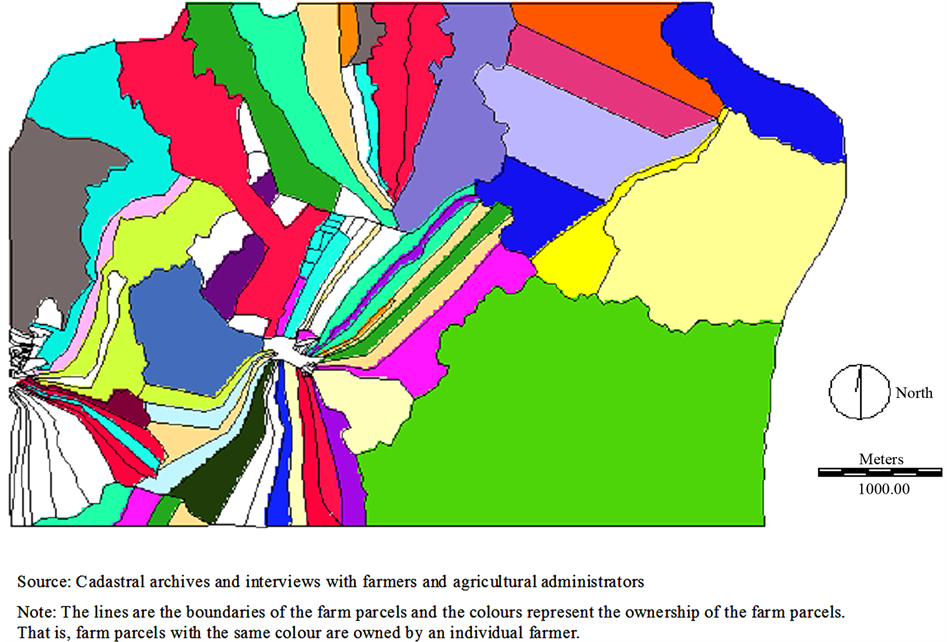
Figure 3. Structure of farm ownerships in the case study area.
cated and somewhat older. Farming activities are less diversified and based on livestock breeding and cereal production. Many active farmers have successors. Unlike the innovative and active farmers, the absentee and retiree farmers are less responsive to changes in their environment. The absentee farmers live further away from the village and their farms are usually managed by neighbouring farmers. Farming is not their main source of income, but the land is retained for personal reasons (e.g. inheritance) or investment purposes. The retiree farmers have the lowest level of education and have the highest average age (76 years). Although they live close to their properties, they no longer farm actively and, consequently, are indifferent to changes in their environment. Their main sources of income are forest subsidies and retirement pensions.
Land use and agricultural suitability: The land use map for the year 2000 is used as an initial condition which changed over time following farmer land use decisions in response to the changing economic and climatic condition. The map was derived from aerial photographs and classified qualitatively on screen by visual interpretation of land cover [33] (Figure 4). The land use pattern is diverse with Montado, forest and arable crops dominating the landscape. There are some shrub lands which are maintained mainly for hunting purposes, especially by large land owners (see section 2). The farmer decisions, which are considered in the model, are for the major land uses such as arable (i.e. wheat, grazing), forest (i.e. holm and cork oak, eucalyptus, pine) and shrubs, as well as livestock (i.e. cattle, pig, sheep) and hunting.
A binomial (or dichotomous) logistic regression analysis was used to develop agricultural suitability maps (see Annex B for the methods and results of the logistic regression). The response variable was the land use, and the predictor variables were maps of potential location criteria (e.g. environmental constraints) for land use. For each land use a binary map was created from an overlay of the 1958 and the 2000 land use maps, for which cells were assigned the value 1 where they had recently established Montado, shrub land, holm oak, or cork oak, and 0 where arable land occurred in both 1958 and 2000. Limiting the 1-values to recently established Montado, shrub land, holm oak and cork oak acknowledges that current-day location criteria for land use conversions aredifferent than in the past. Using unchanged arable land as the 0-value for each land use change makes the location criteria for Montado, shrub land, holm oak, or cork oak comparable. The independent variables for the lo
Table 2.Types and attributes of interviewed farmers in Amendoeira da Serra.
aThe median value of the farm size is100 hectares. Note: ++ cluster occupies the highest share + a high share and—no share out of the total attributes.
gistic regression included biophysical variables such as elevation, slope, aspect, soil depth, texture, and organic carbon. Results of the regressions are shown in Figure 5. The steeper slopes, closer to the river valley have a higher frequency of (recent) shrub land. The statistical probability of shrub land was taken as the inverse of the suitability for arable land. The statistical probability of (recent) Montado is relatively high in most areas. The areas with a high statistical probability for holm oak have a lower probability for cork oak, and vice versa, because the elevation variable has opposing signs in the two models: conversions to cork oak occurred more often on the (more accessible) plateau, while the less profitable holm oak is more often established on the lower lying regions near the Guadiana River. It should be noted that because each map was generated from a different binary logistic regression equation, probabilities do not necessarily sum up to one. For example, areas near the Guadiana River have a high statistical probability for both shrub land and holm oak. This means that these areas are not suitable for arable land (i.e. high shrub land probability), but may still be suitable for holm oak. Conversely, areas that have a low statistical probability in all four maps are considered to be the most suitable for arable cultivation.
Economic and climatic environments: The ABM model was forced with changes in the exogenous variables interpreted for the A1fi socio-economic change scenario. The A1 storyline and scenario family describe a future world of very rapid economic growth, global population that peaks in mid-century and declines thereafter, and the rapid introduction of new and more efficient technologies [35] . Thus, in addition to climatic parameters, theinfluence of technological development on crop yields is also considered in the model. The A1 storyline is di-
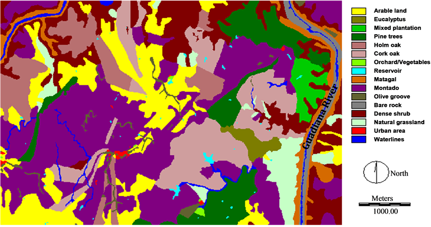
Figure 4. Land use pattern in the case study area 2000.
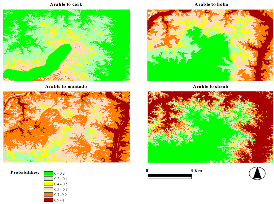
Figure 5. Suitability maps for cork oak, holm oak, Montado and shrubland.
vided into three groups, which are distinguished by their technological emphasis with the A1fi scenario assuming a fossil fuel intensive energy sector. Assumed trends in input and output prices due to market adjustments were used to reflect future changes in the agricultural economy [42] . Changes in the climate and technology were assumed to affect crop yields [37] . The price and yield parameters for Portugal were generated using a stepwise downscaling procedure [35] -[37] [43] . Figure 6 presents the trends in selected socio-economic parameters from 2000 to 2050. In this scenario, the costs of labour are assumed to increase significantly as a result of the assumed movement of young people to urban areas. The costs of other agricultural inputs such as fertilizer and pesticides are assumed to decrease as do the prices of agricultural and livestock products. Yields, however, are assumed to increase significantly as a result of technological development, with the decline in yields due to climate change being offset by the gains derived from technological development. Agriculture is assumed to become less attractive as a source of livelihood because of fewer subsidies for agricultural production and rural development. This discourages land purchase by newcomers and existing land owners, except for innovative farmers. Enlargement of farm size would enable innovative farmers to diversify their production, in particular for hunting purposes.
3.6. Initialisation
The model is initialised by loading the land use map for the year 2000 (Figure 4) and assigning ownership of the farm parcels to the farmers (Figure 3). The socio-economic attributes and typologies of the individual farmers are defined. The variables for the economic environment are initialised using data for the year 2000.
3.7. Submodels
The ABM has four interlinked submodels: 1) typology collectives; 2) ownership collectives; 3) income computation; and 4) adaptive strategies. The UML (Unified Modeling Language) class diagram in Figure 7 shows

Figure 6. Trends in socio-economic and climate-related variables in the A1fi scenario 2000-2050.
the interlinkages between the submodels as well as the components and attributes of each submodel. Land use decisions are mainly a function of farmer type, so the submodel “typology collectives” is an important part of the model. Farmers are classified into one of the four types (retiree, absentee, innovative or active) using the attributes of age, education level (i.e. 0 = none, 1 = 1 - 4 years, 2 = 5 - 6 years, 3 = 7 - 8 years, 4 = advanced studies), location of residence (i.e. 1 = on the property, 2 = in the municipality, 3 = outside the municipality), time spent working on the farm (i.e. 1 = full-time, 2 = part-time), availability of a successor, farm characteristics (i.e. size, suitability) and income level. The characteristics of the farms are defined in the submodel “ownership collectives”. The farms consist of 20 m resolution grid cells and xy-coordinates. Three classes of information are associated with the farms including land use, agricultural suitability and farmer ID. Only crops or farming activities with an agricultural suitability greater than 50% are considered in the land use decisions of the farmers. The grid cells are assigned ID numbers to link them to the farm owners. The farmer IDs are updated annually to account for land that is bought from farmers without a successor (i.e. retiree typology) or who seek non-agricultural employment elsewhere (i.e. active type).
Farmers compute an annual farm income (Equation (1)) in the submodel “income computation”. In the submodel “adaptive strategies”, farmers use the income trend as a basis for changing land use decisions. Farmers engage in repetition if they do not experience a decreasing income trend in the previous years. Otherwise, they engage in maximization or imitation. Maximization is implemented by allowing farmers to evaluate all possible land uses and selecting the one with the maximum income. The income trend is influenced by price, subsidy and yield changes, which are based on the A1fi SRES scenario.
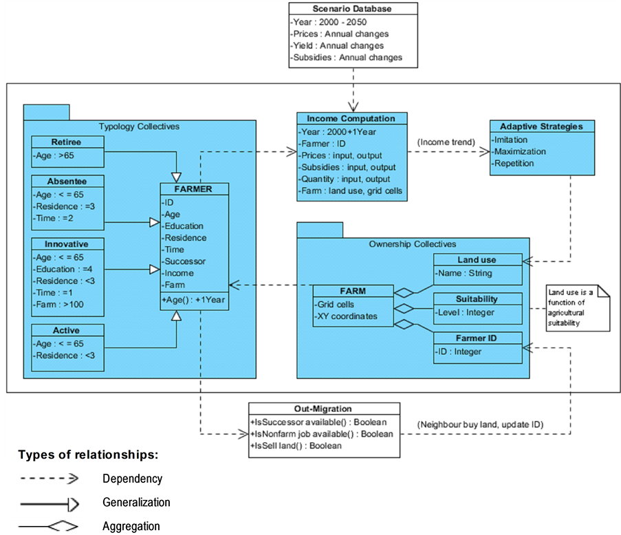
Figure 7. Unified Modeling Language (UML) class diagram of the ABM submodels.
Equation (1)

Where:
INC refers to income;
P refers to prices of m-th output and n-th input in Euro per ton in year T;
Q refers to the quantity of m-th output and n-th input per hectare;
Area refers to the size of the farm in hectares;
FARM refers the farm parcels owned by i-th farmer;
i is the ID of the i-th number of farmer (i = 1, 2, …, 28);
T refers to the number of years (T = 2000, 20001, …, 2050);
c refers to the c-th crop or farm activity.
s.t. is subject to condition that the area belongs to farm parcels of i-th farmer.
Using Equation (1), farmers in the model are assumed to maximize income through simple computation and comparison of profits for alternative, suitable crops. Although this does not involve economic optimization any theoretical limitations of the approach are more than off-set by the analytical and practical advantages for a study of this nature. Economic rationality and optimizing behaviour cannot be assumed when representing individual farmers (rather than generalised individuals) within a study for which diverse decision strategies are known from empirical evidence. In practice, farmers make ad hoc assessments of their costs and returns and employ a range of other decision strategies such as imitation and repetition.
The utility of empirically-grounded models depends on adequate validation and verification [44] . The former checks for the “truthfulness” of the model with respect to its problem domain and the latter the “correctness” of the model construction. ABM verification was conducted through sensitivity and uncertainty analyses. Models that seek to explore future scenarios are impossible to validate completely [37] [44] . Moreover, agent-based models have complex structures that make them difficult to validate as a whole. Alternatively, however, the submodels may be validated individually to ensure that each component represents real system behaviour. The ABM presented here combined statistical relationships with a more process-based simulation of decision-making. An important assumption was that the statistical relationships already include (explicitly or implicitly) all of the processes that lead to the outcome being simulated.
4. Simulation Experiments
Three types of simulations were undertaken: sensitivity, uncertainty and scenario analyses. Sensitivity and uncertainty analysis aim to verify the technical accuracy of the ABM prior to the scenario analysis.
4.1. Sensitivity Analysis
Sensitivity analysis provides information about the input variables that have a major influence on the model outputs [45] [46] . NetLogo’s “BehaviorSpace” integrated software tool was used to run the model several times, systematically varying the values of the input variables and recording the model outputs. This provides an exploration of the model’s possible behaviour space and determines the combinations of settings that cause the behaviour of interest [26] . The sensitivity analysis was based on incremental changes in the income variables including wheat prices, forest subsidies and labour costs and these were mapped against the spatial land use patterns generated by the model for the year 2050. The results of 12 simulations based on ±25% and ±50% changes from the reference values showed that more changes in land use pattern occur when prices and subsidies decrease than when they increase. This is theoretically consistent with the decision rules that farmers change land use when their income decreases. A reduction in arable land due to price changes is accompanied by an increase in Montado. Together with dense shrub, Montado is most sensitive to changes in global (e.g. income) variables.
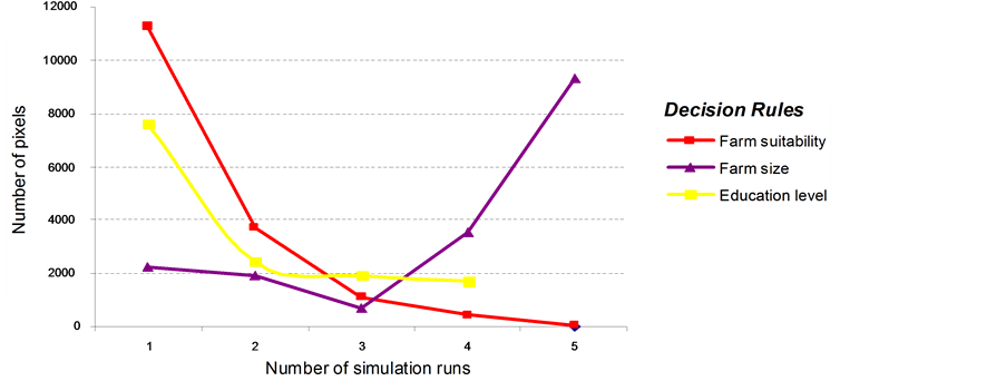
Sensitivity analysis was also undertaken for the decisions rules including farm size, education level, and agricultural suitability. Two types of verification were carried out; changing the decision rules one at a time to verify their individual influence, and changing the decision rules simultaneously to verify the influence of interactions on the model results. For the individual influence verification, five simulations were made for each decision rule, with each run corresponding to incremental changes in their values: education level based on the number of years at school (i.e. 0, 4, 6, 8, and over 8 years); farm size and suitability in increments of 40 hectares and 20 percent, respectively, with a starting value of zero. For the interaction influence verification, the same incremental changes were used (as above), but the values were allowed to change simultaneously in each simulation run. Netlogo’s BehaviorSpace systematically runs the simulation for all combinations of the values for the decision rules. The results of the sensitivity analysis for the individual verification are summarized in Figure 8(a). The direction of change is consistent with the assumptions for all the rules. For example, the number of pixels where land use change occurred decreases as agricultural suitability decreases and increases as farm size increases. This implies that farmers are able to diversify land use as their farm expands. Farm size and suitability have the largest impact on the change in land use with the number of affected pixels (i.e. where land use change occurred) as high as 9000. Figure 8(b) presents the results of the simultaneous verification for the decision rules. Compared with the individual changes in agricultural suitability, farm size, and education level, the combined changes resulted in a larger number of pixels with land use change. For example, for simulation runs with agricultural suitability ranging from 0.20 to 0.60, a farm size of 160 hectares and farmer with lowest education level, land use change occurred in more than 30,000 pixels. Moreover, compared with the results of the individual verification, education level has a greater impact on land use decisions when combined with other rules because the agents can consider various factors in making decisions.
 (a)
(a)  (b)
(b)
Figure 8. Selected results of the sensitivity analyses when the decision rules are modified (a) individually and (b) simultaneously 2050.
Note: The above figures show how land use changes after running the model n-th times (i.e. n = 5 in the upper and n = 27 in the lower figure) when the decision rules are changed one at a time (upper figure) and simultaneously (lower figure). The values of the decision rules used for the n-th simulation runs are between 20 and 100 percent for farm suitability, 50 and 160 hectares for farm size, and 0 and 4 levels for education. The magnitude of land use change is measured from the number of pixels where changes were observed.
4.2. Uncertainty Analysis
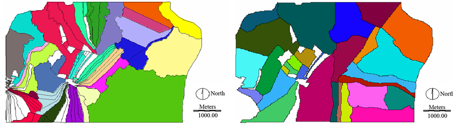
The ABM uses GIS data (e.g. land use, agricultural suitability) and so uncertainty analysis is important in verifying possible errors and uncertainties in the input maps [47] . Such errors may have been generated from classifying land use through remote sensing, identifying farm boundaries with GPS and developing agricultural suitability surfaces with logistic regression. The degree of error propagation and uncertainty was investigated through random distortion of land use and suitability maps and systematic changes in farm size and boundaries, following the methodology proposed by Gómez-Delgado and Bosque Sendra [48] . Here, we present the influence of changing parcel size and boundaries on land use change. New (hypothetical) maps were created for farm ownership as shown in Figures 9(a1) and (b1). Figures 9(a1) shows the actual spatial pattern of farm parcels when farm ownership is reallocated, thus changing the ID number of the farmers. Figure 9(b1) shows a hypothetical spatial pattern of farm parcels following the creation of new farm sizes and boundaries so that farms are either fragmented into several, smaller parcels or clustered into a single, larger parcel.
The results of the uncertainty analysis are presented on the maps in the lower part of Figure 9. Figure 9(a2) refers to the presence or absence of changes in land use resulting from reallocation of actual parcels, while Figure 9(b2) refers to the presence or absence of changes in land use resulting from the creation of the hypothetical spatial pattern of farm parcels. The light shaded areas (in yellow) represent parcels where a change in land use occurred. The results show that land use patterns change with the structure of parcel size and boundaries, and hence with farm ownership. Moreover, when the large parcels were fragmented into smaller parcels, less land use change occurred. In contrast, more land use changes were observed when small parcels were clustered. This implies that as farm size decreases (increases), biophysical constraints increase (decrease) and thus diversification opportunities decrease (increase). Land fragmentation can thus affect ecosystem through reduction in biodiversity. Moreover, land use change depends as much on the socio-economic characteristics of the farmers and
 (a1) (b1)
  (a2) (b2)
Figure 9. Selected results of the uncertainty analyses when (a) actual parcels are clustered and (b) hypothetical parcels are created 2050.
Note: The upper figures are fictitious farm ownerships, which are used to evaluate how property structure affects land use changes. In comparison to farm ownership in Figure 3, the location of ownerships is modified in Figure 8(a1), whilst both spatial pattern and ownership location are modified in Figure 8(b1). As in Figure 3, the colours of the farm parcels depict ownerships. The lower figures show the location of land use changes in 2050 resulting from the modification of the maps of farm ownership from year 2000.
their location in geographic space as on the biophysical characteristics of the farms. This demonstrates that the ABM simulations are only valid for the case study area and that the model could not be generalised to another area or to a larger region even with a similar biophysical environment. In terms of policy implications, this emphasises the need to tie policy measures to the social, economic and cultural values of a local community. Policy measures that aim to conserve traditional landscapes and biodiversity may have different outcomes in areas with similar biophysical characteristics, but different socio-economic conditions.
4.3. Scenario Analysis
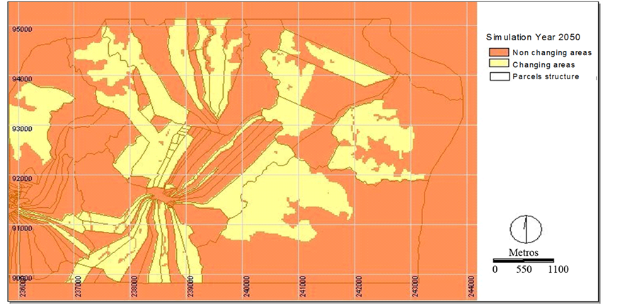
Figure 10(a) presents the spatial location of land use change for the ABM simulations in the year 2050 and Figure 10(b) shows the specific crops contributing to these changes from the year 2000. Under the A1fi scenario, land use change occurs in many parcels (Figure 10(a)) leading to declines in Montado, cork oak and arable land (Figure 10(b)). Compared with the reference year (Figure 4), the land use pattern in 2050 is characterised by an increase in shrub lands and the conversion of forest plantations into unmanaged forests. The increase in both shrub lands and unmanaged forests indicates abandonment of arable and forest plantations, respectively.
 (a)
(a)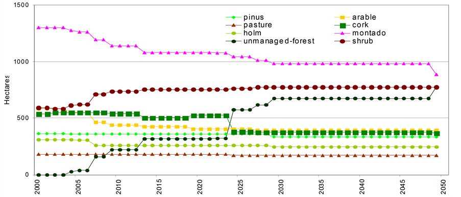 (b)
(b)
Figure 10. Results of scenario analysis-spatial (a) and temporal (b) changes in land use in Amendoiera da Serra 2000-2050.
The A1fi scenario assumes less policy intervention and so farmers receive neither technical advice from agricultural extension services nor subsidies. Consequently, with the exception of innovative farmers, there is no incentive for other farmers to buy the land of active farmers with small and economically unviable farms, or retiree farmers without a successor. In the absence of buyers and successors, lands are abandoned. The lack of agricultural support results in out-migration of farmers particularly those with a higher education level who can find alternative jobs outside the case study area. Abandoned farms remain under the ownership of out-migrating farmers since it is assumed that the state of abandonment is not final or irreversible, and can change when contextual conditions change [49] . Apparently abandoned land in Europe is often not truly abandoned, but temporarily out of use awaiting a new owner or tenant. In the A1fi scenario, it is also assumed that policy does not encourage incomers to buy or lease these temporarily abandoned lands.
Although Montado declines significantly (Figure 10(b)), it remains the dominant land use in 2050 suggesting some resilience to adverse economic and climatic conditions. This is because active farmers who have successors and innovative farmers who support traditional landscapes will continue to maintain their existing Montado. The policy challenge in sustaining Montado in this region beyond 2050 is to encourage a new generation of farmers who recognise not only the economic, but also the social and ecological values of these traditional agricultural landscapes. However, the negative image of agriculture in the Alentejo may limit the effectiveness of economic incentives (e.g. higher agricultural wages or subsidies) in encouraging farmers to stay in the region [7] . The Alentejo was declared officially to be a “particularly disadvantaged region” with Portugal’s entry into the EU in 1986, characterised by labour-intensive and low production agricultural systems resulting in growing migration from the inland areas of Portugal [7] [50] . The decline in population and thus labour supply further contributes to increasing production costs (de Graaff and Eppink 1999 as cited in [51] ).
5. Discussion and Conclusions
The results of the model show that farmers will continue to abandon their land in the future should global economic environment characterised by rapid industrialisation and urbanisation persist. Land abandonment can cause not only social problems (i.e. a decrease in population and loss of cultural identity), but also ecological problems. It constrains the multi-functionality of agro-ecosystems [52] and increases the risk of fires in unmanaged forests due to the accumulation of dead wood [5] [7] [51] , particularly with an increase in drought intensity arising from climate change. Frequent or intense fires can kill adult cork oak trees and affect the persistence of traditional Mediterranean landscapes [5] . Increases in shrub land areas can, however, provide opportunities for nature conservation and leisure amenities. Indeed, the traditional agricultural systems with oaks that have persisted during the 20th century have passed through cycles of use and abandonment (Gallego and Garcia Novo 1997 as cited in [3] ). Abandonment can improve soil conditions and encourage natural vegetation species (annuals and perennials), which tend to minimize soil erosion [53] . Abandonment may improve landscape heterogeneity, and thus biodiversity, through the creation of landscape mosaics that are relatively poor in species, but highly diverse [54] . Shrub land that appears to be abandoned has uses such as beekeeping, hunting and grazing, [55] , particularly by other farmers who have access to neighbouring farmlands that are not enclosed [49] . Farm abandonment is one of the main reasons for the systematic overestimation of pasture land and the underestimation of woodland in census data in Portugal [52] . Economic incentives alone may be insufficient to encourage people to remain in the most isolated Alentejo villages [4] . More innovative and sustainable policy strategies are necessary to encourage the use of abandoned lands in a disadvantaged region like Alentejo. Policy has recently been introduced to support the production of second generation bioenergy crops in the EU. Some of these crops (e.g. short rotation coppice, perennial grasses) are suitable for marginal agricultural lands [56] -[58] and have potential in areas such as Amendoiera da Serra. However, the economic, social and environmental sustainability of bioenergy production remains an important policy challenge [59] -[61]. Bioenergy requires a local market and biomass processing capabilities, but if these were to be available bioenergy production would contribute social and employment benefits to local communities.
Because the area used in this study is relatively small, the model is empirically-grounded with almost all of the individual farmers represented in the model as parameterised agents. Thus, unlike many ABM applications, the model did not use virtual agents and so analysis is based on empirical simulations. Whilst models with virtual agents are useful for testing new concepts, they are not appropriate for testing the land use change implications of policy decisions. The model was also applied at a high spatial resolution that gives the analysis an improved level of realism with agricultural suitability being estimated from biophysical properties that vary greatly with location. Thus the ABM approach makes it possible to retain location specific information in the analysis of complex decision-making process. However, the simulation experiments using different decision rules and different ownership maps demonstrated limitations in generalising the ABM. Thus, applying the model to another geographic location or to a wider society may be difficult. This is because, as the model simulations revealed, knowledge about land use decisions (i.e. farmer attributes and types) and spatial structure (i.e. farm ownership and suitability) needs to be synchronised. The ABM approach is also well suited to the representation of the non-linear dynamics that arise from farmer interactions such as imitation, from the evolution of agent-environment relationships and from the change in agent types and their capacity to learn through time. These types of feedback processes are increasingly important when running simulations over long time periods into the future in response to changing environmental conditions.
Although the scenario analysis presented here is useful in drawing conclusions about the impacts on land use change of perturbations in socio-economics, climate and policy, further applications of the model could usefully compare land use change across a range of plausible scenarios. Analysing scenarios with different assumptions about social behaviour and relationships would be useful in exploring the effects of social networks on land use change. Moreover, because ABM can accommodate a wide range of information types, it can simulate the impacts of both long-term policy objectives such as climate mitigation and short-term policy measures such as rural development. In these types of policy simulations, however, representing soil and vegetation dynamics in response to land use decisions would be a valuable addition, including physical change processes such as soil degradation. This is however beyond the scope of this paper and recommended to be an important component in future research.
Acknowledgements
This research was funded through the VISTA Project that was carried out by the authors at the Département de Géologie et de Géographie, Université catholique de Louvain, Belgium. VISTA was funded within the 5th Framework Programme of the European Commission. We would like to thank Frank Ewert for his support in developing the downscaled economic and climatic scenarios for Portugal.
References
- Costa, A., Pereira, H. and Madeira, M. (2009) Landscape Dynamics in Endangered Cork Oak Woodlands in Southwestern Portugal (1958-2005). Agroforestry Systems, 77, 83-96. http://dx.doi.org/10.1007/s10457-009-9212-3
- Pinto-Correia, T., Ribeiro, N. and Sá-Sousa, P. (2011) Introducing the Montado, the Cork and Holm Oak Agroforestry System of Southern Portugal. Agroforestry Systems, 82, 99-104. http://dx.doi.org/10.1007/s10457-011-9388-1
- Vicente, á.M. and Alés, R.F. (2006) Long Term Persistence of Dehesas. Evidences from History. Agroforestry Systems, 67, 19-28. http://dx.doi.org/10.1007/s10457-005-1110-8
- Pinto-Correia, T. and Vos, W. (2004) Multifunctionality in Mediterranean Landscapes-Past and Future. In: Jongman, R., Ed., The New Dimensions of the European Landscape, Springer, Wageningen, 135-164.
- Acácio, V., Holmgren, M., Moreira, F. and Mohren, G.M. (2010) Oak Persistence in Mediterranean Landscapes: The Combined Role of Management, Topography and Wildfires. Ecology and Society, 15, 40.
- Castro, M. (2008) Silvopastoral Systems in Portugal: Current Status and Future Prospects. In: Rigueiro-Rodríguez, A., Ed., Agroforestry in Europe: Current Status and Future Prospects, Springer Science+Business Media B.V., Berlin, 111-127.
- Santos, M.J. and Thorne, J.H. (2010) Comparing Culture and Ecology: Conservation Planning of Oak Woodlands in Mediterranean Landscapes of Portugal and California. Environmental Conservation, 37, 155-168. http://dx.doi.org/10.1017/S0376892910000238
- Joffre, R., Rambal, S. and Ratte, J.P. (1999) The Dehesa System of Southern Spain and Portugal as a Natural Ecosystem Mimic. Agroforestry Systems, 45, 57-79. http://dx.doi.org/10.1023/A:1006259402496
- Blondel, J. (2006) The “Design” of Mediterranean Landscapes: A Millennial Story of Humans and Ecological Systems during the Historic Period. Human Ecology, 34, 713-729. http://dx.doi.org/10.1007/s10745-006-9030-4
- Matthews, R., Gilbert, N., Roach, A., Polhill, J. and Gotts, N. (2007) Agent-Based Land-Use Models: A Review of Applications. Landscape Ecology, 22, 1447-1459. http://dx.doi.org/10.1007/s10980-007-9135-1
- Valbuena, D., Verburg, P.H. and Bregt, A.K. (2008) A Method to Define a Typology for Agent-Based Analysis in Regional Land-Use Research. Agriculture, Ecosystems and Environment, 128, 27-36. http://dx.doi.org/10.1016/j.agee.2008.04.015
- Janssen, M.A. and Ostrom, E. (2006) Empirically Based, Agent-Based Models. Ecology and Society, 11, 37-49.
- Huigen, M.G. (2004) First Principles of the MameLuke Multi-Actor Modelling Framework for Land Use Change, Illustrated with a Philippine Case Study. Journal of Environmental Management, 72, 5-21. http://dx.doi.org/10.1016/j.jenvman.2004.01.010
- Acosta-Michlik, L. and Espaldon, V. (2008) Assessing Vulnerability of Selected Farming Communities in the Philippines Based on a Behavioural Model of Agent’s Adaptation to Global Environmental Change. Global Environmental Change, 18, 554-563. http://dx.doi.org/10.1016/j.gloenvcha.2008.08.006
- Valbuena, D., Verburg, P.H., Bregt, A.K. and Ligtenberg, A. (2009) An Agent-Based Approach to Model Land-Use Change at a Regional Scale. Landscape Ecology, 25, 185-199. http://dx.doi.org/10.1007/s10980-009-9380-6
- Mena, C.F., Walsh, S.J., Frizzelle, B.G., Yao, X.Z. and Malanson, G.P. (2011) Land Use Change on Household Farms in the Ecuadorian Amazon: Design and Implementation of an Agent-Based Model. Applied Geography, 31, 210-222. http://dx.doi.org/10.1016/j.apgeog.2010.04.005
- Naivinit, W., Page, C.L., Trébuil, G. and Gajaseni, N. (2010) Participatory Agent-Based Modeling and Simulation of Rice Production and Labor Migrations in Northeast Thailand. Environmental Modelling & Software, 25, 1345-1358. http://dx.doi.org/10.1016/j.envsoft.2010.01.012
- Polhill, J.G., Sutherland, L. and Gotts, N.M. (2010) Using Qualitative Evidence to Enhance an Agent-Based Modelling System for Studying Land Use Change. Journal of Artificial Societies and Social Simulation, 13, 10.
- Saqalli, M., Gérard, B., Bielders, C. and Defourny, P. (2010) Testing the Impact of Social Forces on the Evolution of Sahelian Farming Systems: A Combined Agent-Based Modeling and Anthropological Approach. Ecological Modelling, 221, 2714-2727. http://dx.doi.org/10.1016/j.ecolmodel.2010.08.004
- Máñez Costa, M.A., Moors, E.J. and Fraser, E.D. (2011) Socioeconomics, Policy, or Climate Change: What Is Driving Vulnerability in Southern Portugal? Ecology and Society, 16, 28.
- Oliveira, R. (1998) Causas para a desflorestação e degradação da floresta—Estudo-caso para o concelho de MértolaPortugal. Catena, 12-13, 75-93.
- Carolino, J. (2010) The Social Productivity of Farming: A Case Study on Landscape as a Symbolic Resource for PlaceMaking in Southern Alentejo, Portugal. Landscape Research, 35, 655-670. http://dx.doi.org/10.1080/01426397.2010.519437
- Fragoso, R., Marques, C., Lucas, M.R., Martins, M.D. and Jorge, R. (2009) The Economic Effects of Common Agricultural Policy Trends on Montado Ecosystem in Southern Portugal. Technology p. 21, évora.
- Grimm, V., Berger, U., Bastiansen, F., Eliassen, S., Ginot, V., Giske, J., Goss-custard, J., Grand, T., Heinz, S.K., Huse, G., Huth, A., Jepsen, J.U., Jørgensen, C., Mooij, W.M., Muller, B., Peer, G., Piou, C., Railsback, S.F., Robbins, A.M., Robbins, M.M., Rossmanith, E., Ruger, N., Strand, E., Souissi, S., Stillman, R.A., Vabø, R., Visser, U. and Deangelis, D.L. (2006) A Standard Protocol for Describing Individual-Based and Agent-Based Models. Ecological Modelling, 198, 115-126. http://dx.doi.org/10.1016/j.ecolmodel.2006.04.023
- Grimm, V., Berger, U., Deangelis, D.L., Polhill, J.G., Giske, J. and Railsback, S.F. (2010) The ODD Protocol: A Review and First Update. Ecological Modelling, 221, 2760-2768. http://dx.doi.org/10.1016/j.ecolmodel.2010.08.019
- Wilensky, U. (1999) NetLogo, Center for Connected Learning and Computer-Based Modeling Northwestern University, Evanston, IL. Center for Connected Learning and Computer-Based Modeling. Northwestern University, Evanston.
- Railsback, S.F., Lytinen, S.L. and Jackson, S.K. (2006) Agent-Based Simulations Platforms: Review and Development Recommendations. Simulation, 82, 609-623. http://dx.doi.org/10.1177/0037549706073695
- Allan, R.J. (2010) Survey of Agent Based Modelling and Simulation Tools. Technical Report DL-TR-2010-007, Science and Technology Facilities Council (STFC), Warrington WA4 4AD, 48.
- Bakker, M.M. and van Doorn, A.M. (2009) Farmer-Specific Relationships between Land Use Change and Landscape Factors: Introducing Agents in Empirical Land Use Modelling. Land Use Policy, 26, 809-817. http://dx.doi.org/10.1016/j.landusepol.2008.10.010
- Acosta-Michlik, L. and Rounsevell, M. (2005) From Generic Indices to Adaptive Agents: Shifting Foci in Assessing Vulnerability to the Combined Impacts of Climate Change and Globalization. IHDP Update 01, 14-16.
- Grothmann, T. and Patt, A. (2005) Adaptive Capacity and Human Cognition: The Process of Individual Adaptation to Climate Change. Global Environmental Change, 15, 199-213. http://dx.doi.org/10.1016/j.gloenvcha.2005.01.002
- Jager, W., Janssen, M.A., Vries, H.D., Greef, J.D. and Vlek, C. (2000) Behaviour in Commons Dilemmas: Homo economicus and Homo psychologicus in an Ecological-Economic Model. Ecological Economics, 35, 357-379. http://dx.doi.org/10.1016/S0921-8009(00)00220-2
- van Doorn, A.M. and Bakker, M.M. (2007) The Destination of Arable Land in a Marginal Agricultural Landscape in South Portugal: An Exploration of Land Use Change Determinants. Landscape Ecology, 22, 1073-1087. http://dx.doi.org/10.1007/s10980-007-9093-7
- Bakker, M.M., Govers, G., Kosmas, C., Vanacker, V., Oost, K.V. and Rounsevell, M. (2005) Soil Erosion as a Driver of Land-Use Change. Agriculture, Ecosystems & Environment, 105, 467-481. http://dx.doi.org/10.1016/j.agee.2004.07.009
- Nakicenovic, N., Alcamo, J., Davis, G., de Vries, B., Fenhann, J., Gaffin, S., Gregory, K., Grübler, A., Jung, T., Kram, T., Emilio La Rovere, E., Michaelis, L., Mori, S., Morita, T., Pepper, W., Pitcher, H., Price, L., Riahi, K., Roehrl, A., Rogner, H., Sankovski, A., Schlesinger, M.E., Shukla, P., Smith, S., Swart, R., Van Rooyen, S., Victor, N. and Dadi, Z. (2000) Special Report on Emissions Scenarios. Cambridge University Press, Cambridge, 570.
- Rounsevell, M.D., Ewert, F., Reginster, I., Leemans, R. and Carter, T.R. (2005) Future Scenarios of European Agricultural Land Use: II. Projecting Changes in Cropland and Grassland. Agriculture, Ecosystems and Environment, 107, 117-135. http://dx.doi.org/10.1016/j.agee.2004.12.002
- Rounsevell, M., Berry, P.M. and Harrison, P.A. (2006) Future Environmental Change Impacts on Rural Land Use and Biodiversity: A Synthesis of the ACCELERATES Project. Environmental Science & Policy, 9, 93-100. http://dx.doi.org/10.1016/j.envsci.2005.11.001
- Schröter, D., Acosta-Michlik, L., Arnell, A., Araújo, M., Badeck, F. and Bakker, M. (2004) Advanced Terrestrial Ecosystem Analysis and Modelling (ATEAM). Final Report 2004, Potsdam Institute for Climate Impact Research (PIK). Potsdam.
- Carmona, A., Nahuelhual, L., Echeverría, C. and Báez, A. (2010) Linking Farming Systems to Landscape Change: An Empirical and Spatially Explicit Study in Southern Chile. Agriculture, Ecosystems and Environment, 139, 40-50. http://dx.doi.org/10.1016/j.agee.2010.06.015
- Hair, J.F., Anderson, R.E., Tatham, R.L. and Black, W.C. (1995) Multivariate Data Analysis. 4th Edition, Prentice-Hall, Inc., New Jersey, 757.
- Shih, M., Jheng, J. and Lai, L. (2010) A Two-Step Method for Clustering Mixed Categroical and Numeric Data. Tamkang Journal of Science and Engineering, 13, 11-19.
- Abildtrup, J., Audsley, E., Giupponi, C., Gylling, M., Rosato, P. and Rounsevell, M. (2006) Socio-Economic Scenario Development for the Assessment of Climate Change Impacts on Agricultural Land Use: A Pairwise Comparison Approach. Environmental Science & Policy, 9, 101-115. http://dx.doi.org/10.1016/j.envsci.2005.11.002
- Ewert, F., Rounsevell, M.D., Reginster, I., Metzger, M. and Leemans, R. (2005) Future Scenarios of European Agricultural Land Use: I. Estimating Changes in Crop Productivity. Agriculture, Ecosystems and Environment, 107, 101-116. http://dx.doi.org/10.1016/j.agee.2004.12.003
- Parker, D.C., Manson, S.M., Janssen, M.A., Hoffmann, M.J. and Deadman, P. (2003) Multi-Agent Systems for the Simulation of Land-Use and Land-Cover Change: A Review. Annals of the Association of American Geographers, 93, 314-337. http://dx.doi.org/10.1111/1467-8306.9302004
- Saltelli, A., Chan, K. and Scott, E.M. (2009) Sensitivity Analysis. Analysis. John Wiley & Sons LTD, Chichester, 494.
- Gómez Delgado, M. and Tarantola, S. (2006) GLOBAL Sensitivity Analysis, GIS and Multi-Criteria Evaluation for a Sustainable Planning of a Hazardous Waste Disposal Site in Spain. International Journal of Geographical Information Science, 20, 449-466. http://dx.doi.org/10.1080/13658810600607709
- Dendoncker, N., Schmit, C. and Rounsevell, M. (2008) Exploring Spatial Data Uncertainties in Land Use Change Scenarios. International Journal of Geographical Information Science, 22, 1013-1030. http://dx.doi.org/10.1080/13658810701812836
- Gómez Delgado, M. and Bosque Sendra, J. (2009) Validation of GIS-Performed Analysis. In: Joshi, P., Pani, P., Mohapatra, S. and Singh, T., Eds., Geoinformatics for Natural Resource Management, NOVA Publishers, New York, 559571.
- Brouwer, F., van Rheenen, T., Dhillion, S. and Elgersma, A. (2008) Sustainable land Management: Strategies to Cope with the Marginalisation of Agriculture, Strategies. Edward Elgar Publishing Limited, Cheltenham, 252.
- Krauss, W. (2005) Of Otters and Humans: An Approach to the Politics of Nature in Terms of Rhetoric Werner. Conservation and Society, 3, 354-370.
- Duartea, F., Jones, N. and Fleskens, L. (2008) Traditional Olive Orchards on Sloping Land: Sustainability or Abandonment? Journal of Environmental Management, 89, 86-98. http://dx.doi.org/10.1016/j.jenvman.2007.05.024
- Jones, N., Graaff, J.D., Rodrigo, I. and Duarte, F. (2011) Historical Review of Land Use Changes in Portugal (before and after EU Integration in 1986) and Their Implications for Land Degradation and Conservation, with a Focus on Centro and Alentejo Regions. Applied Geography, 31, 1036-1048. http://dx.doi.org/10.1016/j.apgeog.2011.01.024
- Roxo, M. and Casimiro, P. (2004) Desertification Indicator System for Mediterranean Europe DESERTLINKS Project, Land Abandonment: The Lower Inner Alentejo Portugal-Left Bank of the Guadiana River.
- Pinto-Correia, T. (1993) Land Abandonment: Changes in the Land Use Patterns around the Mediterranean Basin. Cahiers Options Méditerranéennes, CIHEAM-IAMZ, Zaragoza, 97-112.
- van Doorn, A.M. and Pinto-Correia, T. (2007) Differences in Land Cover Interpretation in Landscapes Rich in Cover Gradients: Reflections Based on the Montado of South Portugal. Agroforestry Systems, 70, 169-183. http://dx.doi.org/10.1007/s10457-007-9055-8
- Hazell, P. and Pachauri, R.K. (2006) Bioenergy and Agriculture: Promises and Challenges. International Food Policy Research Institute (IFPRI), Washington, 28.
- Cotula, L., Dyer, N. and Vermeulen, S. (2008) Fuelling Exclusion? The Biofuels Boom and Poor People’s Access to Land. IIED, London, 73.
- Dale, V.H., Kline, K.L., Wiens, J. and Fargione, J. (2010) Biofuels: Implications for Land Use and Biodiversity. Ecological Society of America (ESA), Washington DC, 15.
- Acosta-Michlik, L., Lucht, W., Bondeau, A. and Beringer, T. (2011) Integrated Assessment of Sustainability TradeOffs and Pathways for Global Bioenergy Production: Framing a Novel Hybrid Approach. Renewable and Sustainable Energy Reviews, 15, 2791-2809. http://dx.doi.org/10.1016/j.rser.2011.02.011
- Acosta, L.A., Enano, N.H., Magcale-Macandog, D.B., Engay, K.G., Herrera, M.N., Nicopior, O.B., Sumilang, M.I., Eugenio, J.M. and Lucht, W. (2013) How Sustainable Is Bioenergy Production in the Philippines? A Conjoint Analysis of Knowledge and Opinions of People with Different Typologies. Applied Energy, 102, 241-253. http://dx.doi.org/10.1016/j.apenergy.2012.09.063
- Acosta, L.A., Eugenio, E.A., Enano, N.H., Magcale-Macandog, D.B., Vega, B.A., Macandog, P.B.M., Eugenio, J.M.A., Lopez, M.A., Salvacion, A.R. and Lucht, W. (2014) Sustainability Trade-Offs in Bioenergy Development in the Philippines: An Application of Conjoint Analysis. Biomass and Bioenergy, In Press.
Annex A. Cluster Analysis of Farmers’ Socioeconomic Attributes in Amendoeira da Serra
The input variables for the cluster analysis are presented in Table A1. Two-step approach was used for the analysis because as compared to other cluster approaches it can efficiently combine both categorical and continuous dataset. This approach combines both hierarchical and non-hierarchical clustering procedures to arrive at the most realistic cluster solution for the data set. The first step of the cluster analysis aimed to determine the optimal number of clusters evident in the data based on a hierarchical grouping procedure. We used the Ward’s hierarchical clustering method with squared Euclidean distance.
Table A2 presents the agglomeration schedule, which is the result from the first step of the cluster analysis. The schedule shows the changes in the agglomeration coefficients (i.e. the distance between the clusters) at each stage of the clustering procedure. The large increase in the value of the coefficients is a result of joining two different clusters, and thus can be used as an indication of the optimal point to stop merging the clusters [40] . Relatively large percentage increases in the agglomeration coefficients in column 3 are evident between clusters 4 and 3 (14%), between clusters 3 and 2 (16%), and between clusters 2 and 1 (31%). Although the percentage increase between clusters 4 and 5 remains large at 15%, we only considered the first four clusters because including more clusters will result in clusters with few members since there are only 28 farmers. The 2-, 3- and 4-cluster solutions were thus carried over to the second step of the cluster analysis.
Table A1. Variables used as input for the cluster analysis.
Table A2. Agglomeration schedule generated from the first step of the cluster analysis.
In the second step, the cluster centers derived from the hierarchical clustering were used as the initial seed points for the non-hierarchical cluster analysis to achieve maximum grouping efficiency. The K-means clustering approach was performed for the 2-, 3- and 4-cluster solutions. Because the K-means procedure calculates the distances of the clusters to the cluster centroid until the best possible cluster centre is achieved (i.e. when cluster centres are farthest from one another), we investigated the relative differences in the Euclidean distance values between the various cluster solutions. The resulting Euclidean distances of the clusters in each of the cluster solutions in Table A3 show that the 4-cluster solution has cluster centres that are farthest from one another. The average distance for the 4-cluster solution is 77.84, while those for the 2- and 3-cluster solutions are only 71.36 and 67.25, respectively. These results confirm that the data set is best represented with four clusters. The cluster analysis was carried out using the SPSS software.
Table A3. Euclidean distances generated from the second step of the cluster analysis.
Annex B. Binomial logistic Regression to Generate Probabilities of Land Conversion in Amendoeira da Serra
A binomial or dichotomous logistic regression analysis was applied to identify the extent to which the land-use decisions of the farmers in the past were associated with various biophysical properties. The biophysical properties, which are the independent variables for the logistic regression, include biophysical variables such as elevation, slope, south exposition, soil depth, texture, and organic carbon. The dependent variables are the land-use changes, which take two possible values—1 = change and 0 = no change. Four types of land use change were modelled separately including 1) arable to holm oak; 2) arable to cork oak; 3) arable to Montado; and 4) arable to shrub (matorral species). These are the four dominating land use in the case study area from 1958 to 2000 in the village of Amendoeira da Serra. Van Doorn and Bakker [33] investigated the land use changes and developed land use maps through qualitative classification of aerial photographs and visual interpretation of land cover for years 1958, 1969, 1985, 1990 and 2000. For the purpose of the logistic regression, we adopted the land use maps for 1958 and 2000 because they produce the highest possible number of observed changes, in particular for Montado (Figure B1), which is the focus of the analysis in this paper. A large number of observations are necessary to produce estimates from the regression analysis with good statistical fit. As shown in the figure, arable land was continuously declining during these five periods. There was no adequate numbers of observations to implement regression models of land use conversion from arable to other crops.
The logistic model describing the probability of a land-use change (i.e. Pr(change)) can be represented by the following equations:
Equation (1) 
Equation (2) 
Equation (1) defines the probability of land-use change as a function of k explanatory variables. Equation (2) presents an alternative way of formulating the logistic model using the logit form. The logit is a transformation of the probability Pr(change) to make the model linear [62] . Four types of land use change were modelled separately including arable to holm oak, arable to cork oak, arable to Montado, and arable to shrub. These land use changes occurred frequently in the study area during the study period. For each land use change a binary map was created from an overlay of the 1958 and the 2000 land use maps, wherein “change” observations were assigned the value 1 and all “no-change” observations (i.e. unchanged arable land) were assigned the value 0.
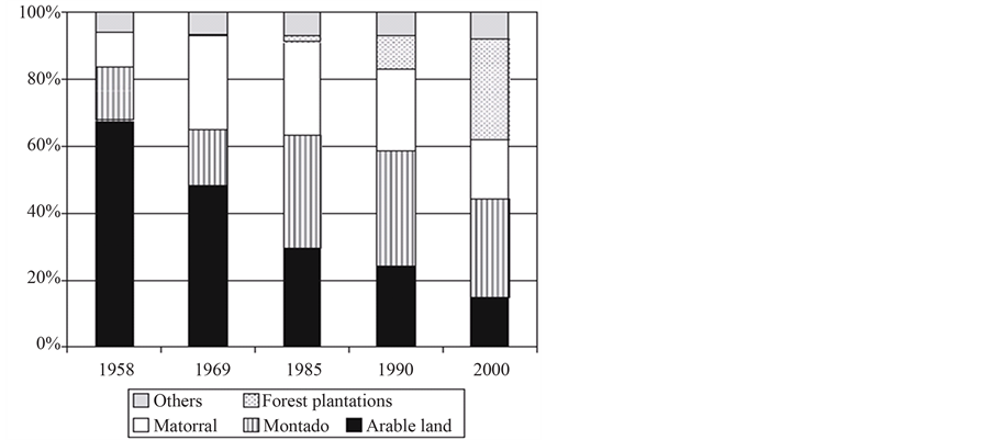
Figure B1. Changes in land cover/use over the time period 1958-2000, Amendoeira da Serra, Source: Van Doorn, A.M. and Bakker, M., 2007 [33] .
Occurrences of land use (change) irrelevant to the particular model (e.g. “unchanged holm oak” or “from cork oak to Montado”) were assigned “no data”. These maps were combined in a GIS with maps of the potential explanatory variables. All maps had a resolution of 20 m. The four regression models were calibrated on a stratified sample drawn from the GIS maps (one observation per hectare). The models were analysed using the SPSS software.
Only the biophysical variables were used as explanatory variables because the socio-economic variables such as farmers’ age, education, etc. are relatively dynamic over time. Compared with the socio-economic variables, the biophysical variables barely change over time, so they are assumed to represent the situation prior to the land use changes. Since the observations of the socio-economic variables do not stem from the period prior to the land use changes, they are not suitable as explanatory variables in the regression analysis. However, the relationships between the socio-economic and biophysical variables were not entirely ignored. The interaction between the socio-economic characteristics of the farmers and the biophysical characteristics of their farms was modelled endogenously in the ABM. Because independent parameters for each of the socio-economic and biophysical variables are needed as input data to the ABM, it is important that these variables are not correlated. Where the socio-economic characteristics of the farmers did correlate with the biophysical characteristics, the observed associations between land use change and the biophysical variables may be biased because the socio-economic variables are taken into account twice: first, in the ABM, where they should be taken into account, and secondly, via the relationship between land use and biophysical properties. Hence, the relationships between land use and the biophysical properties could be taken as a proxy for the socio-economic characteristics of the farmers. Finally, an analysis of the same dataset in another study by Bakker and Van Doorn [29] reports that correlations between socio-economic characteristics and biophysical characteristics are largely absent.
Table B1 presents the results of the regression models. The regression coefficients of the biophysical variables define the contribution of each explanatory variable to a particular land use change. For example, with each degree increase of slope the probability of converting land from arable to shrub increases with . The spatial pattern of the probabilities (i.e. the relative influence of the explanatory variables) was assumed to remain constant over time. Although technological development could change the relative importance of the individual variables to the probability, it was difficult to take this factor into consideration due to lack of data for the case study area. However, due to the relevance of technologies on land-use decisions, the future impacts of technology were directly taken into account in the ABM model through changes in yields based on IPCC SRES scenarios.
Table B1. Results of the regression analysis for land use change in Amendoeira da Serra.
Note: The variables are selected using a backward selection procedure and all the variables listed above have a confidence interval of more than 95%.