Intelligent Information Management
Vol.2 No.3(2010), Article ID:1484,5 pages DOI:10.4236/iim.2012.23023
A New Numerical Method for Solving the Stokes Problem Using Quadratic Programming
Department of Mathematics, Ferdowsi University of Mashhad, Mashhad, Iran
E-mail: mhbaymani@yahoo.com, krachian@math.um.ac.ir
Received December 24, 2009; revised January 28, 2010; accepted March 1, 2010
Keywords: Galerkin Method, Neural Network Model, Quadratic Programming Problem, Stokes Problem
Abstract
In this paper we present a new method for solving the Stokes problem which is a constrained optimization method. The new method is simpler and requires less computation than the existing methods. In this method we transform the Stokes problem into a quadratic programming problem and by solving it, the velocity and the pressure are obtained.
1. Introduction
Developing solutions to the Stokes equations has attracted many researchers because of its practical importance in the field of fluid mechanics. However, due to the nonlinear nature of Stokes equations the main stream of the solutions procedures are in fact numerical methods, which have been developed considerably in recent years because of the amazing advances in computing power and speed. However, very limited information is available in the form of analytical functions as the Stokes solutions especially, when the nonlinear terms remain in the governing equations.
Numerical approximation of incompressible flows presents a major difficulty, namely, the need to satisfy a compatibility condition between the discrete velocity and pressure spaces [1–3]. This condition which has been well known since the work of Babuska and Brezzi prevents, in particular, the use of equal order interpolation spaces for the two variables, which is the most attractive choice from a computational point of view.
To overcome this difficulty, stabilized finite element methods that circumvent the restrictive inf_sup condition have been developed for Stokes-like problems (see [4–6]). These residual-based methods represent one class of stabilized methods. They consist in modifying the standard Galerkin formulation by adding mesh-dependent terms, which are weighted residuals of the original differential equations. Although for properly chosen stabilization parameters these methods are well posed for all velocity and pressure pairs, numerical results reported by several researchers seem to indicate that these methods are sensitive to the choice of the stabilization parameters. The local stabilization suggested in [6] has some advantages in this regard. Another class of stabilized methods has been derived using Galerkin methods enriched with bubble functions (see [7,8]). Alternative stabilization techniques based on a continuous penalty method have been proposed and analyzed in [9,10]. Nafa and Wathen analyzed pressure stabilized finite element methods for the solution of the generalized Stokes problem and investigated their stability and convergence properties. An important feature of the method is that the pressure gradient unknowns can be eliminated locally thus leading to a decoupled system of equations [11].
This paper is devoted to the Stokes system of differential equations. The Stokes problem describes the motion of an incompressible viscous fluid in a 2-dimensional domain:
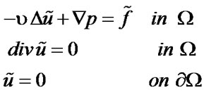 (1)
(1)
here  is the velocity field and
  is the pressure. The first equation is the (linearized) momentum equation, while the second equation expresses the incompressibility constraint. Since we are assuming that the fluid is incompressible, no sources or sinks are present. The given external force field
  causes an acceleration of the flow. The pressure gradient gives rise to an additional force which prevents a change in the density. If (1) is satisfied by some functions
  and
and  then we call
  and
and  a classical solution of the Stokes problem. Note that (1) only determines the pressure
  up to an additive constant, which is usually fixed by enforcing the normalization [1].
2. Mathematical Formulation an Analysis
We assume that , and set
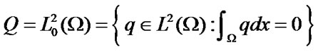

which are Hilbert spaces.
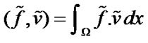
From the first equation of (1) and Green's formulae we obtain
 (2)
(2)
where
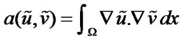
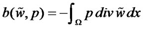 and
and
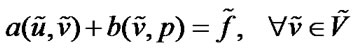
Thus we have the variational form of the problem (1) as:
find 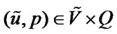 such that
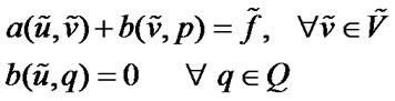 (3)
(3)
In the following we state some conditions and theorems about the stability and convergence of the problem.
Definition: The bilinear forms
are called continuous if they satisfy
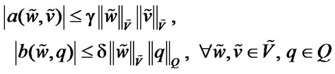 (4)
(4)
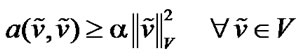
Also  is coercive if there exists a constant
  such that
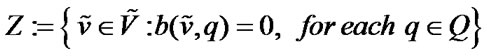
We let
Theorem 1. (Existence and uniqueness) Assume that the bilinear form  satisfies (4) and coercive on Z, moreover,
  satisfy (4) and that the following compatibility (inf_sup) condition holds i.e., there exists
  such that
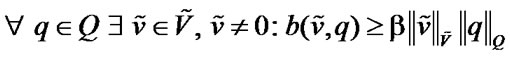 (5)
(5)
Then for each  there exists a unique solution
  and
and
 (6)
(6)
For the proof of the above theorem see [12].
3. Discrete Mixed Formulation
We introduce two families of finite dimensional subspaces  and
and  depending on h. Then, we approximate (3) by the discrete problem: find
 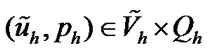 such that
 (7)
(7)
Similar to Z we let
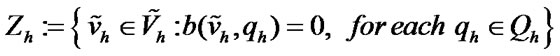
This is the space of discretely divergence-free functions associated with finite dimensional spaces.
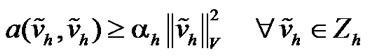
Theorem 2. (Existence and uniqueness) Assume that bilinear forms  and
and  are continuous. The existence and uniqueness of solution to the problem (3) follows from the coercivity of
  on
on  and from discrete inf-sup condition. These two conditions are defined as follows:
There exists a constant  such that
 (8)
(8)
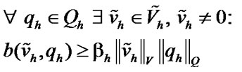 (9)
(9)
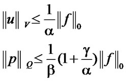
Then for each , there exists a unique solution
  to (7) which satisfies
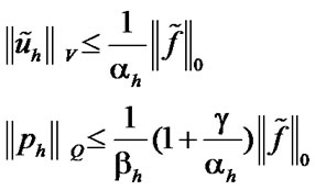
These estimates state that the solution is stable if  is independent of
 . When the latter condition is not true, or even worse, (5) doesn't hold, the approximation (7) is said to be unstable.
Theorem 3. (Convergence) Let the assumptions of Theorems (3) and (4) be satisfied. Then the solutions  and
and  to (3) and (7), respectively, satisfy the following error estimates
 (10)
(10)
Moreover, the following estimate holds
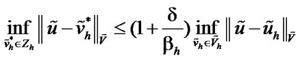 (11)
(11)
From (10) and (11) it follows that the convergence is optimal, provided that (8) and (9) hold with constants independent of  [12,13].
Using basis functions for  and
and , the problem (7) leads to the following system of linear equations:
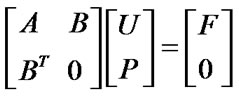 (12)
(12)
where A is a symmetric positive definite matrix. It can be shown that the discrete inf-sup condition is satisfied or this system has a unique solution if and only if  [1,12,13]. If
 , then the coefficient matrix in (12) is singular, and the system has infinitely many solutions. In this case, for solving the system (12), we can use one of the iterative methods or the penalty method.
In this paper, we assume . We introduce the quadratic programming method for solving the Stokes problem.
4. Illustration of the Method
In this section we present an optimization method for solving the problem (3).
Consider the following problem:
 (13)
(13)
The following theorem shows the relation of the solutions of (3) and (13).
Theorem 4. The optimal solution of the optimization system (13) is the unique solution of the problem (3).
Proof: The optimal solution of (13) is  such that
 , then
So, the optimal solution of (13) is the solution of (3).
In the Galerkin method, for solving (7) using finite element approximation requires a lot of computations to construct the space of basis functions ( . But, here we choose the space
  of basis functions easily such that the boundary conditions are satisfied and
 . The new method leads to the solution
 . We approximate the problem (13) by the discrete problem:
find  such that:
 (14)
(14)
Similarity, we can show that the optimal solution of the problem (14) is the solution of discrete form of the problem (9).
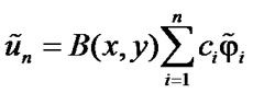
We choose v in the form

where  are independent and
  is a known function such that
  is equal to zero on the boundary. Thus we take the approximation solution
  in the form
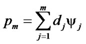
Also, we write the approximation solution  as a linear combination of independent functions
By substituting  and
and  in (14), the optimization problem is transformed into the following quadratic programming:
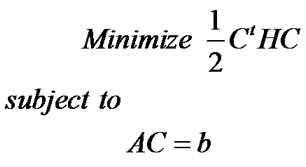 (15)
(15)
where , H is a
  symmetric semi definite matrix, A is a
  matrix.
5. Solving QP Problem
Consider the following QP problem:
 (16)
(16)
where H is an  symmetric positive semidefinite matrix, A is an
  matrix and
 . The Karush-KuhnTucker conditions of the problem (16) are:
 (17)
(17)
For solving the system (17), we use the following neural network model
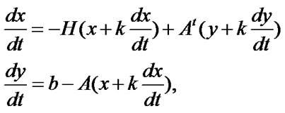 (18)
(18)
The details are given in [14].
6. Numerical Results
Example: We consider the problem (1) with the unit square  and with the following smooth exact solution

We solve this problem by the method described in previous section and use  (polynomials of degree
 ) and
) and  (polynomials of degree
  in each of the variables). This means that
  and
and . Also, we compare our results with least-square finite element ([15]) with
 . The numerical results have been shown in Table 1 for different viscosities.
The errors of the exact and approximation solutions for  are depicted in Figures 1-3.

Table 1. Numerical results.
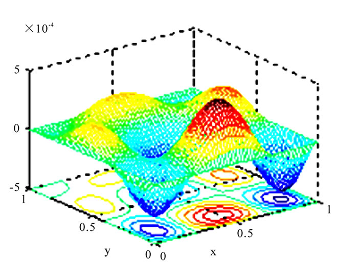
Figure 1. Error function ( ).
).

Figure 2. Error function ( ).
).
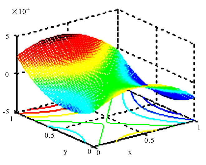
Figure 3. Error function ( ).
).
7. Conclusions
In this paper we transformed the Stokes problem into a quadratic programming problem, and by solving it, we obtained the velocity and pressure as a linear combination of independent functions. The advantages of this method over the usual finite element method are the differentiallity of the approximation solution, and computational work which is less than usual finite element. The performance of the scheme and the accuracy of the results are evaluated by compared with the reliable numerical in literature. The preliminary results presented in this paper show a promising future for the method. Yet more elaborations are required for identifying a systematic way of defining the solution function, which remains for future studies.
8. References
[1] F. Brezzi and M. Fortin, “Mixed and hybrid finite element methods,” Springer-Verlag, New York, 1991.
[2] H. Elman, D. Silvester, and A. Wathen, “Finite elements and fast iterative solvers with applications in incompressible fluid dynamics,” Oxford University Press, Oxford 2005.
[3] V. Girault, and P. Raviart, “Finite element methods for Navier–Stokes equations,” Springer-Verlag, Berlin, 1986.
[4] T. Barth, P. Bochev, M. Gunzburger, and J. Shahid, “A taxomony of consistently stabilized finite element methods for stokes problem,” SIAM Journal on Scientific Computing, Vol. 25, pp. 1585–1607, 2004.
[5] L. P. Franca, T. J. R. Hughes, and R. Stenberg, “Stabilised finite element methods,” in: Incompressible Computational Fluid Dynamics Trends and Advances, Cambridge University, pp. 87–107, 1993.
[6] N. Kechkar and D. Silvester, “Analysis of locally stabilized mixed finite element methods for Stokes problem,” Mathematics of Computation, Vol. 58, pp. 1–10, 1992.
[7] R. Araya, G. R. Barrenechea, and F. Valentin, “Stabilized finite element methods based on multiscale enrichment for the Stokes problem,” SIAM journal on Numerical Analysis, Vol. 44, No. 1, pp. 322–348, 2006.
[8] G. R. Barrenechea and F. Valentin, “Relationship between multiscale enrichment and stabilized finite element methods for the generalized Stokes problem I,” CR Academic Science, Vol. 341, pp. 635–640, 2005.
[9] E. Burman, M. Fernandez, and P. Hansbo, “Continuous interior penalty finite element method for Oseen’s equations,” SIAM Journal on Numerical Analysis, Vol. 44, No. 6, pp. 1248–1274, 2006.
[10] E. Burman and P. Hansbo, “Edge stabilization for the generalized Stokes problem: A continuous interior penalty method,” Computer Methods on Applied Mechanics and Engneering. Vol. 195, pp. 2393–2410, 2006.
[11] K. Nafa, and A. J. Wathen, “Local projection stabilized Galerkin approximations for the generalized Stokes problem,” Computer Methods on Applied Mechanics and Engneering, Vol. 198, pp. 877–883, 2009.
[12] B. Borre and N. Lukkassen, “Application of homogenization theory related to Stokes flow in porous media,” Applications of Mathematics, Vol. 44, No. 4, pp. 309–319, 1999.
[13] A. Quarteroni and A. Valli, “Numerical approximation of partial differential equations,” ISBN 3–540–57111–6, Springer-Verlag, Berlin Heidelberg, New York, 1997.
[14] S. Effati and M. Baymani, “A new nonlinear neural network for solving quadratic programming problems,” Applied Mathematics and Computational, Vol. 165, pp. 719–729, 2005.
[15] C. C. Tsai and S. Y. Yang, “On the velocity-vorticitypressure least–squares finite element method for the stationary incompressible Oseen problem,” Journal of Computational and Applied Mathematics, Vol. 182, pp. 211–232, 2005.