Journal of Geographic Information System
Vol.10 No.01(2018), Article ID:82367,31 pages
10.4236/jgis.2018.101005
Spatial Transferability of Vegetation Types in Distribution Models Based on Sample Surveys from an Alpine Region
Linda Aune-Lundberg1, Anders Bryn2,3
1Division of Survey and Statistics, Norwegian Institute of Bioeconomy Research, Tromsø, Norway
2Division of Survey and Statistics, Norwegian Institute of Bioeconomy Research, Ås, Norway
3Natural History Museum, University of Oslo, Oslo, Norway

Copyright © 2018 by authors and Scientific Research Publishing Inc.
This work is licensed under the Creative Commons Attribution International License (CC BY 4.0).
http://creativecommons.org/licenses/by/4.0/


Received: December 20, 2017; Accepted: February 6, 2018; Published: February 9, 2018
ABSTRACT
Vegetation mapping using field surveys is expensive. Distribution modelling, based on sample surveys, might overcome this challenge. We tested if models trained from sample surveys could be used to predict the distribution of vegetation types in neighbourhood areas, and how reliable the spatial transferability was. We also tested whether we should use ecological dissimilarity or spatial distance to foresee modelling performance. Maximum entropy models were run for three vegetation types based on a vegetation map within a moun- tain range. Environmental variables were selected backwards, model complexity was kept low. The models are based on points from a small part of each study site, transferred into the entire sites, and then tested for performance. Environmental distance was tested using principle component analysis. All models had high uncorrected AUC values. The ability to predict presences correctly was low. The ability to predict absences correctly was high. The ability to transfer the distribution model depended on environmental distance, not spatial distance.
Keywords:
Area Frame Survey, Ecological Distance, GIS, Independent Evaluation Data, Maximum Entropy Modelling, Vegetation Mapping

1. Introduction
Distribution modelling (DM), with the aim of modelling the potential distribution of a target by relating its distribution to environmental variables (EV), has proliferated during the last decades and is increasingly used for spatial predictions within applied ecology [1] [2] . In contrast to process-based mechanistic models used to simulate past, current and future vegetation patterns [3] , DM methods are correlative and therefore less dependent of causal relationships [4] . Most DM studies address the species level, but DM methods are also frequently used in studies that focus on the vegetation, habitat or nature type level [5] [6] [7] , as well as higher levels such as floristic or landscape regions [8] [9] . In this paper, we address DM challenges at the vegetation type level.
Vegetation types represent more or less stable entities of plant communities characterized by physiognomy, plant species composition, indicator species, or a combination of all three, and they are influenced by a number of ecological processes through time and space [10] [11] . Each vegetation type reflects a unique ecological space that sums up the ecological processes which structure the pattern of vegetation at the spatial scale of the applied mapping system [12] . An ecologically well-defined vegetation type is usually found within ecologically similar locations throughout a given geographical domain. A vegetation map therefore represents a spatial generalization of the vegetation structure, classified according to predefined types that intend to mirror the underlying ecological processes at a given spatial scale [6] .
All DM methods are based on spatially explicit presence-points, but some methods also include absence-points (e.g. GLM and GAM). The EVs however, always appear as wall-to-wall maps, with a specified resolution (grain size) and extent [13] . The goal of DM is therefore to fit a model by use of spatially explicit points and EVs to provide wall-to-wall predictions of the potential distribution of the target. In this study, we implement a presence-only (P-O) method which is frequently used for DM, maximum entropy modelling [14] .
Only small fractions of the earth have been mapped through field surveys [11] . On the other hand, the number of coarse-scaled wall-to-wall land cover maps with fewer classes based on remote sensing (RS) has increased tremendously over the last three decades [15] [16] . RS methods have so far not been able to map vegetation types according to the acquired accuracy and level of information for many biodiversity management purposes [17] [18] . This is in particular true for mountain regions at high latitudes where topography, low sun-angle, frequent clouds and a short growing season combine to make RS difficult. Much of the present detailed mapping of vegetation, forest and landscape types is therefore performed by area frame surveys using field work and/or aerial photo interpretation [19] [20] [21] [22] .
Since area frame surveys mostly consist of representative samples, today’s usages are mainly restricted to non-spatial statistical purposes and area resource estimates, e.g. use of small area estimation methods [23] [24] . However, area frame surveys can also serve as DM training sites for vegetation types, if the knowledge of spatial transferability of DM predictions is well consolidated by empirical studies, and errors and uncertainties [25] [26] [27] are well interpreted.
The main aim for this study was to assess spatial transferability of DMs trained by sample P-O points from survey vegetation maps. More specifically, we set out to analyse the following challenges: Can we use DM, fitted with MaxEnt and trained with P-O points generated from a gridded plot-sample survey, to predict the distribution of vegetation types in neighbourhood areas (areas outside the training plot)? How reliable is the spatial transferability of the DM when confronted with independent evaluation data? How and why are prediction performance decreasing as a response to increasing spatial or ecological distance from training plots (within a spatial domain) when DM is applied? Based on environmental indicators representing areas of similar size as the survey plots, but located at increasing spatial distances, can we in advance (by analyses of the ecological space) detect areas of low DM performance?
2. Materials and Methods
2.1. Study Area
The study area covers 941 km2 of the Rondane mountain region in south-central Norway (centre coordinate 548857N/686140E, in WGS84/UTM32N). The topography varies from gently undulating mountain plateaus to high alpine peaks and ranges in elevation from 441 to 2176 m.a.s.l. The mean annual temperature at the closest weather station, Venabu, Ringebu (930 m.a.s.l.), is −0.3˚C (1980- 1990), and mean annual precipitation is 842 mm (2005-2011). The bedrock is completely dominated by acidic Precambrian rocks which are partly covered by thin and discontinuous layers of glacial till [28] . The alpine-boreal vegetation of the study area reflects the continental climate and the varying altitude [29] . The climatic forest line reach 1200 m a.s.l. [30] , but the north boreal zone appear regularly below approximately 1000 m a.s.l.
2.2. Vegetation Map
The vegetation map of the study area was compiled into a seamless map, using results from mapping projects performed between 1980 and 1992 [31] . The guidelines for mapping remained practically unchanged throughout the project period [32] [33] . In the field-guide, there are detailed instructions for a number of difficult aspects [34] . The classification was based on a combination of homogenous species composition, indicator species and vegetation physiognomy. The mapping was validated with extensive field-work and recently updated using high-resolution orthophotos from 2010. The map includes 28 vegetation types and 7 other land cover types (Appendix 1). The seamless map was converted into raster format of 10 m resolution and joined with a digital elevation model (DEM) of equal resolution.
2.3. Vegetation Type Targets
Three vegetation types were chosen as targets; dwarf shrub heaths, tall forb meadows and fens. The choice was based on three requirements; divergent pre- valence within the study area (rare, intermediate and widespread), a widespread distribution pattern, and finally divergent ecology related to well-known EVs that proxies can be generated for. Dwarf shrub heath is very common throughout the study area, whereas fen is broadly distributed, but generally with lower prevalence and smaller occurrences. Tall forb meadows are relatively rare and appear scattered along narrow zones.
2.4. Study Design
The study area was covered by a grid with primary statistical units (PSU) of 1500 m × 600 m, each covering 0.9 km2. This grid is in accordance with the Norwegian area frame survey of land cover and outfield land resources [21] . The three vegetation types were treated independently throughout the study.
For each vegetation type, five sites were randomly positioned within the study area, but restricted to avoid spatial overlap within each targeted vegetation type. Each site was 10,500 m × 9600 m (100.8 km2), consisting of a matrix of 7 × 16 PSUs. A random PSU, including the targeted vegetation type, in one of each site corner was chosen as the model PSU (Figure 1).
Based on the model PSU two transects were created along the outer edge of the sites in two directions, resulting in 105 test PSUs for each vegetation type.
Sets of P-O training points were generated from the vegetation map, one set of the target vegetation type for each of the different model PSUs. To avoid spatial autocorrelation, the training points were extracted from a grid with a mesh size of 20 × 20 m [35] . However, points that include vegetation types in mosaic polygons or in polygons with additional signs originating from a different ecosystem than the vegetation type targeted for modelling were excluded (Appendix 2).
Presence-absence evaluation data were generated from the vegetation map for each PSU using a grid with a mesh size of 10 × 10 m.
For each model PSU the following data is available: Training P-O points used for modelling, presence-absence (P-A) points used for evaluation, sets of EVs, and a DM based on output from MaxEnt. Except for the training points, similar data sets were prepared for all test PSUs. Each PSU contains a total of 9000 points, attributed with P-A and the characteristics for the EVs.
2.5. Environmental Variables (EV)
A DEM, and ten EVs derived from the DEM was used in the study (Table 1). The derived EVs were generated in ArcGIS® 10.1 using Spatial Analysis. These EVs are widely used in ecological studies [36] , and have been reported as relevant for DM of vegetation types in previous studies [6] [37] . The EVs has a resolution of 10 × 10 m. Aspect was used as an ordinal variable, all the other EVs were continuous.
The EVs were tested for correlation (Pearson’s r) and only EVs correlated less than ±0.7 were used in the final DMs (Appendix 3).
Figure 1. The study area in Norway. For each vegetation type; dwarf shrub heath, tall forb meadow and fen, five different non-overlapping study sites were prepared (covering 100.8 km2). The vegetation map, used for evaluation, is shown in the background. Inside each of the study sites a model PSU (0.9 km2), containing the given vegetation type, was chosen randomly located in one of the corners (marked with blue). From the model PSU two transects were created along the outer edge of the study sites (marked with arrows).
Table 1. Environmental variables (EV) considered in the modelling and the ecological factors they were intended as proxies for. EVs finally implemented are marked with grey shading.
2.6. Distribution Modelling Method
Maximum entropy modelling (MaxEnt version 3.3.3k, http://www.cs.princeton.edu/~schapire/maxent/) was used in this study. It is described as a machine learning method [38] , but can also be explained as a maximum likelihood method [39] . Based on P-O records of a specific target and EVs for the study area, MaxEnt creates a prediction model for the distribution of the target using the EVs in the presence-cells as auxiliary support [40] [41] .
The vegetation types was modelled and extrapolated using common MaxEnt modelling strategies, described for instance in [42] . The default settings were overrode and we strived for models that balanced the contradiction between: 1) a low number of parameters by removing features that resulted in high lambdas, 2) as high training AUC values as possible and 3) as few EVs as needed but without removing variables known to be important for modelling of the vegetation types. The goal was to make parsimonious MaxEnt models suitable for spatial transferability [40] [42] .
Based on experiences with the dataset, only linear and quadratic features [14] [38] [41] were allowed. This prevented over-fitted models. Models fit for different number of background samples was compared and the number of background points was set to 1000. The regularization multiplier was set to 0, after testing different options. With just two features and a relatively high number of training points (Table 2) we found this acceptable. Visual inspection of the response curves also indicated smooth curves. For all other settings we used default values.
A backward step-wise selection using the area under the curve values (AUC) [38] , percent contribution of the EVs to the model and jackknife was used to select the included EVs in the final models [39] [43] .
The maximum training sensitivity plus specificity, based on the logistic output format [14] , was used as threshold rule for two reasons; to create a vegetation map that provides presence or absence for all locations of all vegetation types [12] [44] , and as a part of the model evaluation process. The maximum training sensitivity plus specificity was chosen based on the results from several other studies [7] [45] [46] . All relative probability of predicted presence (RPPP) above the threshold was assumed to be the given vegetation type, and the score of correct classification was calculated based on the presence-absence points.
One MaxEnt model was fitted to each of the fifteen different study sites as described above. The MaxEnt models from the different model PSUs were used for projection (transferability) into the adjacent test areas by means of EVs recorded for the latter area.
2.7. Evaluation of the Spatial Transferability
The model output from MaxEnt was evaluated against the P-A evaluation data from the wall-to-wall vegetation map, with the same resolution as the model data from MaxEnt.
The model precision was calculated based on four categories; correct predicted absence, incorrect predicted absence, correct predicted presence and incorrect predicted presence. The accuracy of the MaxEnt models was calculated as the percentage of correct predicted absence and presence against the actual absence and presence. The classification accuracy and error rate was calculated by a confusion matrix using the total number of points inside the four different categories for each of the three different vegetation types.
We tested if the DM could be used to predict absence and presence for the three given vegetation types using the ± standard error interval (SE). The null hypothesis (H0) was that the percentage of each of the four categories used for evaluation of the MaxEnt models was zero.
Potential difference in the accuracy of prediction for absence and presence were tested by the 95% confidence interval (CI) of the difference between correct predicted absence and correct predicted presence.
2.8. Ecological Distance
The ecological distance was based on the EVs used in the MaxEnt models for the different study areas (Table 2). A dissimilarity metrics based on the results from Principal Component Analysis (PCA) [47] was used as a measure for ecological similarity between the test PSUs and the model PSU.
PCA is an indirect ordination method aimed at restructuring complicated data into a manageable format [48] . For PCA we only included EVs used in the MaxEnt model for each vegetation type, and we could not detect convincing arch or horseshoe effects [49] . The different EVs represent units measured on
Table 2. Descriptions of the most important model parameters and the percent contribution of EVs in the final five DM models run for each vegetation type.
unequal scales, so we normalized all variables using division by their standard deviations. Furthermore, we used eigenvalue scales, created 95% concentration ellipses for each PSU (run site by site) and used the information from those ellipses in the further analyses of dissimilarity among PSUs. We used metrics from the 95% ellipses representing the first two PCA axes; mean x and mean y.
To express the dissimilarity among PSUs provided by the PCAs, we used standard Euclidean dissimilarity and distance metrics [48] .
2.9. Evaluation of the Ecological and Spatial Distance
The coherence between the predictions/correct predictions and the ecological and spatial distance was analysed. Spatial distance was set as the Euclidean distance between the midpoint of the model PSU and the midpoint of each of the test PSUs. Ecological distance is described in the above chapter. The correlation between the predicted presence for the three different vegetation types and the ecological and spatial distance was analysed using linear regression analysis. The correct predicted absence and presence data were analysed in the same way.
3. Results
3.1. Descriptions of the Models
A model for each of the different study sites was fitted. Between two and five different EVs were used, see Table 2 for details about the model parameters.
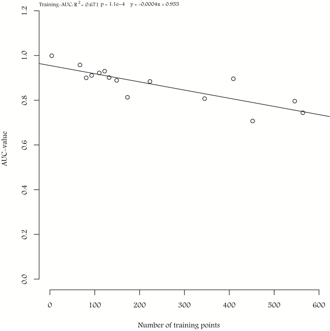
A correlation between the number of training points and the training-AUC value was observed, with a decrease in training-AUC value with an increase in the number of training points (R2 = 0.69, p = 1.1e−4) (Appendix 4).
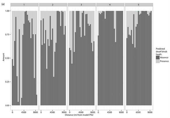
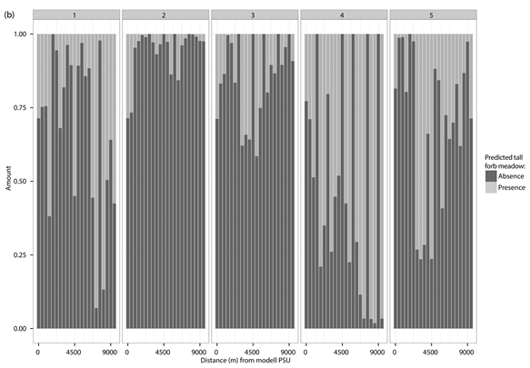
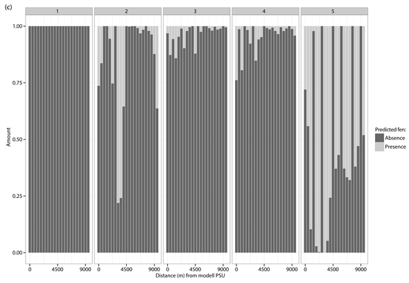
The predicted presence of the types varied widely between the PSUs inside the study sites. The mean predicted percentage coverage for dwarf shrub heath was 19% of the study sites, and the mean predicted percentage coverage for tall forb meadow and fen was 26% and 16%, respectively. The amount of predicted presence for the three different vegetation types ranged from 0% to >98% coverage of the test PSUs (Appendix 5).
3.2. Evaluation of the Spatial Transferability
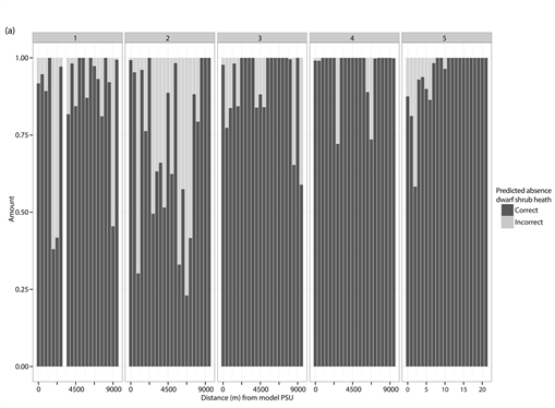
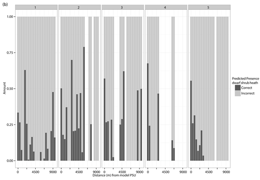
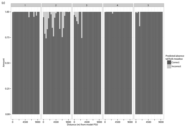
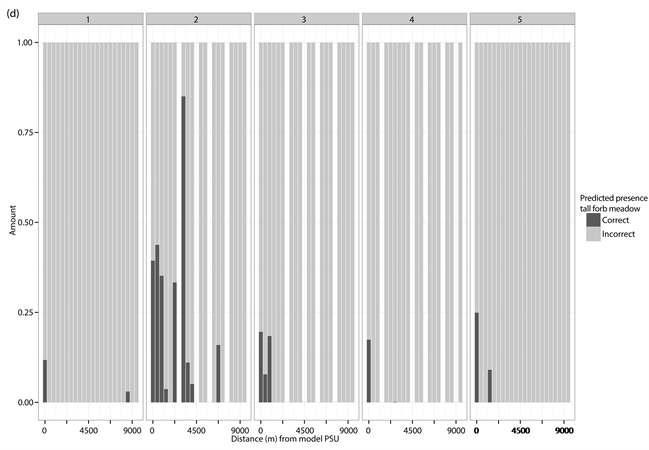
The percentage predicted absence verified as correct is high for all the vegetation types; 90.0% for dwarf shrub heath, 96.9% for tall forb meadow and 97.7% for fen. The percentage predicted presence verified as correct is low; 23.4% for dwarf shrub heath, 1.9% for tall forb meadow and 6.1% for fen (Table 3; Appendix 6).The classification accuracy based on the confusion matrix varies between 76% and 84% for the three different vegetation types.
The H0 was rejected for correct predicted absences and incorrect predicted presences, but was not rejected for correct predicted presences, e.g. the ±SE included zero. There is a significant difference of the model performance between the correctness of prediction of absence and presence for all the vegetation types. The 95% CI of the margins between the amounts of correctly predicted absence
Table 3. Statistics from the verification of the MaxEnt models.
and correctly predicted presence is not close to 0 (Table 3), but is high for all three types.
3.3. Predictions of Vegetation Types vs. Ecological and Spatial Distance
The regression between the amount of predicted presence and ecological and spatial distance is presented in Figure 2. The relationship for the amount of predicted absence is the opposite of the relationship for the amount of predicted presence.
The general tendency is that the number of predicted presence decreases with increasing ecological distance. The increase of spatial distance on the other hand, does not influence the number of predicted presences. The regression for predicted presence vs ecological distance is significant (p < 0.005) for dwarf shrub heath and fen. However, a tendency for decreasing amount of predicted presence with increasing ecological distance is also seen for tall forb meadow (p = 0.07). The regression for the number of predicted presence vs. spatial distance is not significant for tall forb meadow and fen. There is a trend (p = 0.02) that the number of predicted presence decrease with increasing distance from the model PSU for dwarf shrub heath.
For the most common type, dwarf shrub heath, the linear regression between the correct classified presences against both the ecological and spatial distance is significant (p < 0.005); with a decrease in the amount of correct classified presence with an increase of ecological or spatial distance (Figure 3).
The pattern for correct predicted absence is less clear. It is a trend towards a positive correlation between correct predicted absence and ecological distance (p
Figure 2. Linear regression, with 95% CI, for the relationship between predicted presence and ecological distance and spatial distance for three vegetation types. ((a), (b)): Dwarf shrub heath. ((c), (d)): Tall forb meadow. ((e), (f)): Fen.
Figure 3. Linear regression with 95% CI, for the relationship between correct predicted absence and presence and ecological and spatial distance for dwarf shrub heath.
< 0.05), but there is no correlation between correct predicted absence and spatial distance.
The number of correct predicted absence for tall forb meadow shows only a weak tendency for correlation with ecological distance (p < 0.1) and no correlation with spatial distance (Appendix 7). The correct predicted presence shows a significant negative correlation with both ecological and spatial distance (P ≤ 0.005).
There is a significant (p < 0.005) positive correlation between the number of correct classified absence and ecological and spatial distance for fen (Appendix 8). A trend for negative correlation between the number of correct predicted presence and the ecological and spatial distance is seen (P < 0.1).
4. Discussion
4.1. Spatial Transferability of Vegetation Types Using DM
The distribution models resulted in fairly high training AUC-values. Following Araújo, Pearson, Thuiller and Erhard [50] , all the resulting DMs should thus be interpreted as having good predictive ability. In an interpolation setting, a random proportion of the P-O points could have been used as a test data set for evaluation of the model [41] . In studies of spatial transferability, i.e. in an extrapolation setting, such testing is not possible, since there are no P-O points in the projected areas. With the lack of evaluation data it is not possible to state anything certain about the transferability of the models, given that training AUC-values only report the ability of a model to explain the distribution of the training points. When confronted with independent P-A evaluation points from the projected neighbourhood areas, the results revealed several important aspects, but first we need to discuss the specific DM design used in this study.
4.2. Setting the Scene for Spatial Transferability in DM
Provided that the goal of spatial transferability in DM studies is to project the targets relationship to EVs from an informed area into an uninformed area, it is a prerequisite to avoid model over-fitting [51] . This seems to be a general statement valid also for temporal transferability in DM [52] [53] [54] . Therefore, instead of maximizing the fit to the particular training P-O points of each PSU, we reduced the model fit and complexity. In transferability studies, such choices depend on a priori knowledge with the DM method [14] , the ecology of the target and the environmental variation within the area for projection [27] . In retrospect, given the results of implementing the P-A evaluation points, it is of course unproblematic to acknowledge that changes in for example model fitting or binary threshold rules could have improved the results. However, we have not included any a posteriori corrections according to the results, since the goal was to test the spatial transferability using a real dataset and a realistic departure point for DM, rather than to train for the ‘best’ modelling setup as an iterative process [55] .
4.3. Ecological Dissimilarity―Not Spatial Distance
A fundamental assumption in spatial analysis (sensu lato) is Tobler’s first law of geography [56] [57] . A priori, we therefore expected a gradually decreasing DM performance with increasing distance from the training PSUs, in accordance with the results of other studies [e.g. [51] ].
In this study, the overall proportion of predicted presences did not change much with increasing spatial distance (Figure 2), but the variation was high. The high variation indicate high environmental turnover within and among the PSUs, which was better described by the ecological distance provided by PCA. Thus, instead of defining spatially coherent domain(s) for DM projection at regional-to-global scale [e.g. 51], the ecological dissimilarity within each cell should define ecologically coherent domain(s) (Figure 4). We recommend excluding all cells that are ecologically too dissimilar compared with the ecology of the training site, regardless of spatial distance.
Elith, Kearney and Phillips [58] warned against using DM in environmental novel areas outside the range of training values by implementing a measure of environmental similarity (MESS). We used the variation along the first two axes of PCA to extract the most structuring environmental novelty, which in DM often is well described by a very limited number of EVs [35] , to evaluate the spatial transferability. The methods have differences, but in our opinion, the strong correlation between correctly predicted cells and ecological distance in our study, strongly supports the warning of Elith et al. [58] and others [59] .
4.4. Confronting DMs with Independent P-A Evaluation Data
Confronting the predictions with independent evaluation data reveals that the specificity is high, but the sensitivity is low. The total classification accuracy is relatively high for the three vegetation types (Table 3), which we judge to be a result of high specificity and large areas with absence of the targets. Given that the DMs identify areas of true absence, it should be a logical consequence that it was also able to identify areas of true presence. However, our results point at the fact that we have a precise modelling of absence, but an un-precise modelling of
Figure 4. Visualization of potential domains based on spatial distance (a) and ecological distance (b).
presence. The DM is thus guiding us to the relevant areas of potential presence, but with a low spatial accuracy. If we had implemented a different binary threshold rule and kept the same model settings, the RPPP values and DM results would not have changed, but it could have displayed the proportions of predicted absence and presence differently. Having the results of the independent test, the negative correlation between the amount of correctly predicted pre- sence and the ecological and spatial distance, enables the possibility to use a binary threshold rule that increase the sensitivity of the models. However, without the independent test, we would not have known a priori which of the binary threshold rules to implement.
The effects of ecological and spatial distance changes when the predictions are confronted with independent evaluation data. The correctly predicted presence for all types is negatively correlated with the ecological as well as the spatial distance. No such clear pattern is observed for the correctly predicted absence. The correlation between the predicted presence and ecological and spatial distances (Figure 2) gives a picture based on the MaxEnt models alone; the EVs and the training data. The real situation, when the model data are confronted with the evaluation data, reveals a more complex picture, where undetected ecological factors influence the results. The absence of the vegetation types can be seen as a diverse group, whereas the presence is more homogeneous.
4.5. Sources of Error and Uncertainties
Although topographic EVs derived from DEMs have been found to be highly useful for DM studies [1] and have shown to explain the local distribution of some vegetation types [6] [60] , they do not represent the entire ecological signature needed to predict the vegetation types in question. In the absence of high resolution climate data, we have used altitude as a collective climate proxy, well aware of the uncertainties related with the use of this confounding EV [61] . We believe the DM presented in this study could have been improved by adding several relevant EVs, such as snow cover, temperature, precipitation (sensu lato), and soil macronutrients. These EVs however, was not available or only available at irrelevant resolution. For the purpose of DM, we acknowledge that several missing EVs could have improved the in situ model fit, but they would most likely not have improved the spatial transferability. The main source of error for spatial transferability of DMs is in our opinion the lack of environmental variation represented by the training P-O points in relation to a more varied environment within the area intended for projection.
The overall results for the three vegetation types were congruent, but some differences were identified. The locally common vegetation type fen performed best of the tested vegetation types. The distribution of fens is clustered, and the total cover is relatively low. Dwarf shrub heath is the most common vegetation type, both in extent and distribution, and the internal variability is high [62] . The extrapolation of the vegetation type achieved an intermediate result, but was more accurately modelled than seen in earlier studies [6] . The locally and overall rare tall forb meadow resulted in the lowest accuracy model, and was largely overestimated. We acknowledge two main reasons for this. First; the vegetation type requires plenty of soil nutrients and moisture [33] . Second; it is a possibility that the vegetation type has too low prevalence to be predicted precisely. Based on only three vegetation types with varying prevalence and ecology, we would warn about drawing too general conclusions.
4.6. Practical Implications
In this study we have only tested local transferability of a DM based on sample survey data. The results did not support our initial intention to use the DM framework as a substitute for vegetation mapping, since the models were better at recognizing absences than presences. However, if sample survey data were to be implemented as a practical part of DM for vegetation mapping, presence data from all sampled survey plots would be activated simultaneously. That would imply a shift from DM based on local spatial extrapolation sensu stricto, to DM based on interpolation among plots in the interior of the extent. This alternative approach raises several new research questions that needs to be addressed, such as; are the provided density (or size) of survey plots high enough to represent both the total and the continuously environmental variation of the vegetation types within the extent, and are rare vegetation types clustered in space (non-random distribution) well represented in the gridded sample survey. These questions will have to be accounted for, before any conclusions can be drawn regarding implementation of DM as a method for vegetation mapping based on area frame survey data.
5. Conclusions
This study has demonstrated several aspects of caution that needs to be handled when DMs of vegetation types, trained with survey data and fitted with MaxEnt, are used for spatial transferability:
・ Area frame surveys of vegetation types, where sample plots are assumed to be representative for a larger spatial domain, should be used with caution in transferability studies using DM.
・ The training P-O points have to be representative for the environmental variation in the area intended for projection.
・ The parameterization, selection of EVs, and model specification will influence the ability to transfer the DM. Based on the low ability to correctly model presences; we believe that under-fitting is influencing the results. It is therefore important to balance the model fit and complexity between the two contrasting goals: to enable a spatial projection of the DM (low model fit), but at the same time, keep a high predictability of presences (high model fit).
・ The transferability of the DMs did not depend on the spatial distance, but correlated well with PCA-indicators of ecological distance among the test sites. The challenge of DM transferability is therefore not primarily to define a spatial domain, but a matter of defining an ecological domain suitable for spatial projection.
・ The reliability of a spatially projected DM can only be addressed thoroughly when tested against independent evaluation data. The training AUC-values from the DMs, did not provide a good estimate of the true modelling performance.
This research was deliberately limited in scope to an examination of data from an existing area frame survey of vegetation types with respect to the spatial transferability of DM fitted with MaxEnt. The focus on the chosen vegetation type data, DM method, EVs and spatial scale however, provides only a certain part of the challenges involved in DM transferability. Nevertheless, as high quality vegetation maps remain a key tool for nature management [43] , and field- work mapping is time-consuming and expensive, we need a better understanding of how to model the distribution of vegetation types from existing data, such as area frame surveys [21] . Spatial modelling techniques, such as the DM methods (e.g. MaxEnt), are increasingly accessible to researchers and should be used to explore the potential for modelling the distribution of vegetation types in areas not yet mapped by traditional methods [6] .
Acknowledgements
Many thanks to Geir-Harald Strand and Rune Halvorsen for valuable comments on a previous version of this article. This article has been financially supported by the Norwegian Institute of Bioeconomy Research and the Natural History Museum (University of Oslo).
Cite this paper
Aune-Lundberg, L. and Bryn, A. (2018) Spatial Transferability of Vegetation Types in Distribution Models Based on Sample Surveys from an Alpine Region. Journal of Geographic Information System, 10, 111-141. https://doi.org/10.4236/jgis.2018.101005
References
- 1. Guisan, A. and Zimmermann, N.E. (2000) Predictive Habitat Distribution Models in Ecology. Ecological Modelling, 135, 147-186. https://doi.org/10.1016/s0304-3800(00)00354-9
- 2. Yackulic, C.B., Chandler, R., Zipkin, E.F., Royle, J.A., Nichols, J.D., Grant, E.H.C. and Veran, S. (2013) Presence-Only Modelling Using MAXENT: When Can We Trust the Inferences? Methods in Ecology and Evolution, 4, 236-243. https://doi.org/10.1111/2041-210x.12004
- 3. Scheiter, S., Langan, L. and Higgins, S.I. (2013) Next-Generation Dynamic Global Vegetation Models: Learning from Community Ecology. New Phytologist, 198, 957-969. https://doi.org/10.1111/nph.12210
- 4. Dormann, C.F., Schymanski, S.J., Cabral, J., Chuine, I., Graham, C., Hartig, F., Kearney, M., Morin, X., Rommermann, C., Schroder, B. and Singer, A. (2012) Correlation and Process in Species Distribution Models: Briding a Dichotomy. Journal of Biogeography, 39, 2119-2131. https://doi.org/10.1111/j.1365-2699.2011.02659.x
- 5. Miller, J., Franklin, J. and Aspinall, R. (2007) Incorporating Spatial Dependence in Predictive Vegetation Models. Ecological Modelling, 202, 225-242. https://doi.org/10.1016/j.ecolmodel.2006.12.012
- 6. Ullerud, H.A., Bryn, A. and Klanderud, K. (2016) Distribution Modeling of Vegetation Types in the Boreal-Alpine Ecotone. Applied Vegetation Science, 19, 528-540. https://doi.org/10.1111/avsc.12236
- 7. Weber, T.C. (2011) Maximum Entropy Modeling of Mature Hardwood Forest Distribution in four U.S. States. Forest Ecology and Management, 261, 779-788. https://doi.org/10.1016/j.foreco.2010.12.009
- 8. Moriondo, M., Jones, G.V., Bois, B., Dibari, C., Ferrise, R., Trombi, G. and Bindi, M. (2013) Projected Shifts of Wine Regions in Response to Climate Change. Climatic Change, 119, 825-839. https://doi.org/10.1007/s10584-013-0739-y
- 9. Zhang, M.-G., Zhou, Z.-K., Chen, W.-Y., Silk, J.W.F., Cannon, C.H. and Raes, C.H. (2012) Using Species Distribution Modeling to Improve Conservation and Land Use Planning of Yunnan, China. Biological Conservation, 153, 257-264. https://doi.org/10.1016/j.biocon.2012.04.023
- 10. Biondi, E., Feoli, E. and Zuccarello, V. (2004) Modelling Environmental Responses of Plant Associations: A Review of Some Critical Concepts in Vegetation Study. Critical Reviews in Plant Sciences, 23, 149-156. https://doi.org/10.1080/07352680490433277
- 11. Millington, A.C. and Alexander, R.W. (2000) Vegetation Mapping in the Last Three Decades of the Twentieth Century. In: Alexander, R.W. and Millington, A.C., Eds., Vegetation Mapping, John Wiley & Sons, Chichester, 321-331.
- 12. Pedrotti, F. (2013) Plant and Vegetation Mapping. Springer Verlag, Heidelberg. https://doi.org/10.1007/978-3-642-30235-0
- 13. Yackulic, C.B. and Ginsberg, J.R. (2016) The Scaling of Geographic Ranges: Implications for Species Distribution Models. Landscape Ecology, 31, 1195-1208. https://doi.org/10.1007/s10980-015-0333-y
- 14. Merow, C., Smith, M.J. and Silander, J.A. (2013) A Practical Guide to MaxEnt for Modeling Species’ Distributions: What It Does, and Why Inputs and Settings Matter. Ecography, 36, 1-12. https://doi.org/10.1111/j.1600-0587.2013.07872.x
- 15. Hussain, M., Chen, D., Cheng, A., Wei, H. and Stanley, D. (2013) Change Detection from Remotely Sensed Images: From Pixel-Based to Object-Based Approaches. ISPRS Journal of Photogrammetry and Remote Sensing, 80, 91-106. https://doi.org/10.1016/j.isprsjprs.2013.03.006
- 16. Walker, D.A., Raynolds, M.K., Daniels, F.J.A., Einarsson, E., Elvebakk, A., Gould, W.A., Katenin, A.E., Kholod, S.S., Markon, C.J. and Yurtsev, B.A. (2005) The Circumpolar Arctic Vegetation Map. Journal of Vegetation Science, 16, 267-282. https://doi.org/10.1111/j.1654-1103.2005.tb02365.x
- 17. Ihse, M. (2007) Colour Infrared Aerial Photography as a Tool for Vegetation Mapping and Change Detection in Environmental Studies of Nordic Ecosystems: A Review. Norwegian Journal of Geography, 61, 170-191. https://doi.org/10.1080/00291950701709317
- 18. Lindgaard, A. and Henriksen, S. (2011) The 2011 Norwegian Red List for Ecosystems and Habitat Types. Norwegian Biodiversity Information Centre, Trondheim.
- 19. Dramstad, W.E., Fjellstad, W.J., Strand, G.H., Mathiesen, H.F., Engan, G. and Stokland, J.N. (2002) Development and Implementation of the Norwegian Monitoring Programme for Agricultural Landscapes. Journal of Environmental Management, 64, 49-63. https://doi.org/10.1006/jema.2001.0503
- 20. Gallego, F.J. and Delincé, J. (2010) The European Land Use and Cover Area-Frame Statistical Survey. In: Benedetti, R., Bee, M., Espa, G. and Piersimoni, F., Eds., Agricultural Survey Methods, Wiley, Chichester, 149-168. https://doi.org/10.1002/9780470665480.ch10
- 21. Strand, G.-H. (2013) The Norwegian Area Frame Survey of Land Cover and Outfield Land Resources. Norwegian Journal of Geography, 67, 24-35. https://doi.org/10.1080/00291951.2012.760001
- 22. Timonen, J., Siitonen, J., Gustafsson, L., Kotiaho, J., Stokland, J., Sverdrup-Thygeson, A. and Mokkonen, M. (2010) Woodland Key Habitats in Northern Europe: Concepts, Inventory and Protection. Scandinavian Journal of Forest Research, 25, 309-324. https://doi.org/10.1080/02827581.2010.497160
- 23. Gallego, F.J. and Bamps, C. (2008) Using CORINE Land Cover and the Point Survey LUCAS for Area Estimation. International Journal of Applied Earth Observation and Geoinformation, 10, 467-475. https://doi.org/10.1016/j.jag.2007.11.001
- 24. Strand, G.-H. and Aune-Lundberg, L. (2012) Small-Area Estimation of Land Cover Statistics by Post-Stratification of a National Area Frame Survey. Applied Geography, 32, 546-555. https://doi.org/10.1016/j.apgeog.2011.06.006
- 25. Jiménez-Valverde, A., Ecevedo, P., Barbosa, A.M., Lobo, J.M. and Real, R. (2013) Discrimination Capacity in Species Distribution Models Depends on the Representativeness of the Environmental Domain. Global Ecology and Biogeography, 22, 508-516. https://doi.org/10.1111/geb.12007
- 26. Thuiller, W., Brotons, L., Araújo, M.B. and Lavorel, S. (2004) Effects of Restricting Environmental Range of Data to Project Current and Future Species Distributions. Ecography, 27, 165-172. https://doi.org/10.1111/j.0906-7590.2004.03673.x
- 27. Wiens, J.A., Stralberg, D., Jongsomjit, D., Howell, C.A. and Snyder, M.A. (2009) Niches, Models, and Climate Change: Assessing the Assumptions and Uncertainties. Proceedings of the National Academy of Sciences, 106, 19729-19736. https://doi.org/10.1073/pnas.0901639106
- 28. Ramberg, I.B., Bryhni, I. and Nøttvedt, A. (2007) The Making of a Land: Geology of Norway. Geological Society of Norway, Trondheim.
- 29. Bakkestuen, V., Erikstad, L. and Halvorsen, R. (2008) Step-Less Models for Regional Environmental Variation in Norway. Journal of Biogeography, 35, 1906-1922. https://doi.org/10.1111/j.1365-2699.2008.01941.x
- 30. Aas, B. and Faarlund, T. (2000) Forest Limits and the Subalpine Birch Belt in North Europe with a Focus on Norway. AmS-Varia, 37, 103-147.
- 31. Rekdal, Y. (1994) Vegetasjonskart, Rondane nasjonalpark. Korrigert utgave [Vegetation Map, Rondane National Park. Corrected Edition]. Norwegian Institute of Land Inventory, Ås.
- 32. Larsson, J. (1974) Vegetasjonskartlegging M 1:50000. Inventering av arealressurser [Vegetation Mapping in Scale 1:50000. Inventory of Area Resources]. Jorddirektoratet, Ås.
- 33. Rekdal, Y. and Larsson, J.Y. (2005) Veiledning i vegetasjonskartlegging [Instruction Manual in Vegetation Mapping] (Report No. 5). Norwegian Institute of Land Inventory, Ås. http://www.skogoglandskap.no/filearchive/Rapport_05_05.pdf
- 34. Bryn, A., Kristoffersen, H.P., Angeloff, M., Nystuen, I., Aune-Lundberg, L., Endresen, D., Svindseth, C. and Rekdal, Y. (2015) Location of Plant Species in Norway Gathered as a Part of a Survey Vegetation Mapping Programme. Data in Brief, 5, 589-594. https://doi.org/10.1016/j.dib.2015.10.014
- 35. Halvorsen, R., Mazzoni, S., Dirksen, J.W., Næsset, E., Gobakken, T. and Ohlson, M. (2016) How Important Are Choice of Model Selection Method and Spatial Autocorrelation of Presence Data for Distribution Modelling by MaxEnt? Ecological Modelling, 328, 108-118. https://doi.org/10.1016/j.ecolmodel.2016.02.021
- 36. Huggett, R. and Cheesman, J. (2002) Topography and the Environment. Prentice Hall, Harlow.
- 37. Hemsing, L.Ø. and Bryn, A. (2012) Three Methods for Modelling Potential Natural Vegetation (PNV) Compared: A Methodological Case Study from South-Central Norway. Norwegian Journal of Geography, 66, 11-29. https://doi.org/10.1080/00291951.2011.644321
- 38. Phillips, S.J., Anderson, R.P. and Schapire, R.E. (2006) Maximum Entropy Modeling of Species Geographic Distributions. Ecological Modelling, 190, 231-259. https://doi.org/10.1016/j.ecolmodel.2005.03.026
- 39. Halvorsen, R., Mazzoni, S., Bryn, A. and Bakkestuen, V. (2014) Opportunities for Improved Distribution Modelling Practice via a Strict Maximum Likelihood Interpretation of MaxEnt. Ecography, 38, 172-183. https://doi.org/10.1111/ecog.00565
- 40. Elith, J., Phillips, S.J., Hastie, T., Dudik, M., Chee, Y.E. and Yates, C.J. (2011) A Statistical Explanation of MaxEnt for Ecologists. Diversity and Distributions, 17, 43-57. https://doi.org/10.1111/j.1472-4642.2010.00725.x
- 41. Phillips, S.J. and Dudik, M. (2008) Modeling of Species Distributions with Maxent: New Extensions and a Comprehensive Evaluation. Ecography, 31, 161-175.
- 42. Merow, C., Smith, M.J., Edwards, T.C., Guisan, A., McMahon, S.M., Norman, S., Thuiller, W., Wüest, R.O., Zimmermann, N.E. and Elith, J. (2014) What Do We Gain from Simplicity versus Complexity in Species Distribution Models? Ecography, 37, 1267-1281. https://doi.org/10.1111/ecog.00845
- 43. Franklin, J. (2009) Mapping Species Distributions: Spatial Inference and Prediction. Cambridge University Press, Cambridge. https://doi.org/10.1017/cbo9780511810602
- 44. Küchler, A.W. and Zonneveld, I.S. (1988) Vegetation Mapping. Kluwer, Dordrecht. https://doi.org/10.1007/978-94-009-3083-4
- 45. Jimenez-Valverde, A. and Lobo, J.M. (2007) Threshold Criteria for Conversion of Probability of Species Presence to Either or Presence-Absence. Acta Oecologica, 31, 361-369. https://doi.org/10.1016/j.actao.2007.02.001
- 46. Liu, C., White, M. and Newell, G. (2013) Selecting Thresholds for the Prediction of Species Occurrence with Presence-Only Data. Journal of Biogeography, 40, 778-789. https://doi.org/10.1111/jbi.12058
- 47. Gardener, M. (2014) Community Ecology. Analytical Methods Using R and Excel. Pelagic Publishing, Exeter.
- 48. Krebs, C.J. (1998) Ecological Methodology. 2nd Edition, Addison Wesley Longman, Menlo Park.
- 49. Karadzic, B. (1999) On Detrending in Correspondence Analysis and Principal Component Analysis. Ecoscience, 6, 110-116. https://doi.org/10.1080/11956860.1999.11952201
- 50. Araújo, M.B., Pearson, R.G., Thuiller, W. and Erhard, M. (2005) Validation of Species-Climate Impact Models under Climate Change. Global Change Biology, 11, 1504-1513. https://doi.org/10.1111/j.1365-2486.2005.01000.x
- 51. Fernández, P., Jordano, D. and Haeger, J.F. (2015) Living on the Edge in Species Distribution Models: The Unexpected Presence of Three Species of Butterflies in a Protected Area in Southern Spain. Ecological Modelling, 312, 335-346. https://doi.org/10.1016/j.ecolmodel.2015.05.032
- 52. Moreno-Amat, E., Mateo, R.G., Nieto-Lugilde, D., Morueta-Holme, N., Svenning, J.-C. and García-Amorena, I. (2015) Impact of Model Complexity on Cross-Temporal Transferability in Maxent Species Distribution Models: An Assessment Using Paleo-Botanical Data. Ecological Modelling, 312, 308-317. https://doi.org/10.1016/j.ecolmodel.2015.05.035
- 53. Warren, D.L. and Seifert, S.N. (2011) Ecological Niche Modeling in Maxent: The Importance of Model Complexity and the Performance of Model Selection Criteria. Ecological Applications, 21, 335-342. https://doi.org/10.1890/10-1171.1
- 54. Warren, D.L., Wright, A.N., Seifert, S.N. and Shaffer, H.B. (2014) Incorporating Model Complexity and Spatial Sampling Bias into Ecological Niche Models of Climate Change Risks Faced by 90 California Vertebrate Species of Concern. Diversity and Distributions, 20, 334-343. https://doi.org/10.1111/ddi.12160
- 55. Guisan, A., Broennimann, O., Engler, R., Vust, M., Yoccoz, N.G., Lehmann, A. and Zimmermann, N.E. (2006) Using Niche-Based Models to Improve the Sampling of Rare Species. Conservation Biology, 20, 501-511. https://doi.org/10.1111/j.1523-1739.2006.00354.x
- 56. Miller, H.J. (2004) Tobler’s First Law and Spatial Analysis. Annals of the Association of American Geographers, 94, 284-289. https://doi.org/10.1111/j.1467-8306.2004.09402005.x
- 57. Tobler, W.R. (1970) A Computer Movie Simulating Urban Growth in the Detroit Region. Economic Geography, 46, 234-240. https://doi.org/10.2307/143141
- 58. Elith, J., Kearney, M. and Phillips, S. (2010) The Art of Modelling Range-Shifting Species. Methods in Ecology and Evolution, 1, 330-342. https://doi.org/10.1111/j.2041-210x.2010.00036.x
- 59. Saupe, E.E., Barve, V., Myers, C.E., Soberón, J., Barve, N., Hensz, C.M., Peterson, A.T., Owens, H.L. and Lira-Noriega, A. (2012) Variation in Niche and Distribution Model Performance: The Need for a Priori Assessment of Key Causal Factors. Ecological Modelling, 237-238, 11-22. https://doi.org/10.1016/j.ecolmodel.2012.04.001
- 60. Oddershede, A., Svenning, J.-C. and Damgaard, C. (2015) Topographically Determined Water Availability Shapes Functional Patterns of Plant Communities within and across Habitat Types. Plant Ecology, 216, 1231-1242. https://doi.org/10.1007/s11258-015-0504-6
- 61. Korner, C. (2007) The Use of “Altitude” in Ecological Research. Trends in Ecology and Evolution, 22, 569-574. https://doi.org/10.1016/j.tree.2007.09.006
- 62. Aune-Lundberg, L. and Strand, G.-H. (2017) Composition and Spatial Structure of Dwarf Shrub Heath in Norway. Norwegian Journal of Geography, 71, 1-11. https://doi.org/10.1080/00291951.2017.1291536
Appendix 1
1Rekdal, Y. (1994) Vegetasjonskart, Rondane nasjonalpark. Korrigert utgave [Vegetation Map, Rondane National Park. Corrected Edition].Norwegian Institute of Land Inventory, Ås.
Distribution of vegetation types within the study area used for model evaluation. The vegetation type classification is based on reference1. Vegetation types used for DM are marked with grey shading. The occurrence of each type is given in km2 and the proportion in percent.
Appendix 2
2Rekdal, Y. (1994) Vegetasjonskart, Rondane nasjonalpark. Korrigert utgave [Vegetation map, Rondane national park. Corrected edition].Norwegian Institute of Land Inventory, Ås.
List of additional information codes used in the vegetation mapping in Norway2. Additional information included in the model points are listed first and additional information not included in the model points are listed last.
Appendix 3
Correlation matrix of the environmental variables considered in the study. Numbers provide Pearson’s product- moment coefficient (r). Correlations above 0.7 are shaded.
Appendix 4
Correlation between the number of training points in the PSUs used for the modelling of the different study sites and the training-AUC values. The linear regression between the number of training points and training-AUC values are marked with a straight line.
Appendix 5
The percentage distribution of predicted presences (light grey) and absences (dark grey) for each of the different test PSUs inside of the different vegetation types and study sites. (a) Dwarf shrub heath; (b) Tall forb meadow; (c) Fen. The test PSUs are sorted in increasing distance from the model PSU.
Appendix 6
The percentage distribution of correct (dark grey) and incorrect (light grey) predicted presences and absences for each of the different test PSUs inside of the different vegetation types and study sites. (a) Correct and incorrect predicted absences for dwarf shrub heath; (b) Correct and incorrect predicted presences for dwarf shrub heath; (c) Correct and incorrect predicted absences for tall forb meadow; (d) Correct and incorrect predicted presences for tall forb meadow; (e) Correct and incorrect predicted absences for fen; (f) Correct and incorrect predicted presences for fen. The test PSUs are sorted in increasing distance from the model PSU. Missing bars indicate no predictions for absences or presences in the given study site.
Appendix 7
Linear regression with 95% CI, for the relationship between correct predicted absence and presence and ecological and spatial distance for tall forb meadow. The predicted presence is reported as the percentage in each test PSU. Ecological distance is derived by the dissimilarity matrix, based on the PCAs of the EVs used in the MaxEnt modelling, and gives the ecological difference between the training points and the test PSUs.
Appendix 8
Linear regression with 95% CI, for the relationship between correct predicted absence and presence and ecological and spatial distance for fen. The predicted presence is reported as the percentage in each test PSU. Ecological distance is derived by the dissimilarity matrix, based on the PCAs of the EVs used in the MaxEnt modelling, and gives the ecological difference between the training points and the test PSUs.


