Natural Science
Vol.6 No.4(2014), Article ID:43344,13 pages DOI:10.4236/ns.2014.64024
Polyhedral symmetry and quantum mechanics
![]()
Institute of Nuclear and Particle Physics, National Center for Scientific Research, Demokritos, Greece; anagnos4@otenet.gr
Copyright © 2014 G. S. Anagnostatos. This is an open access article distributed under the Creative Commons Attribution License, which permits unrestricted use, distribution, and reproduction in any medium, provided the original work is properly cited. In accordance of the Creative Commons Attribution License all Copyrights © 2014 are reserved for SCIRP and the owner of the intellectual property G. S. Anagnostatos. All Copyright © 2014 are guarded by law and by SCIRP as a guardian.
Received 2 December 2013; revised 2 January 2014; accepted 9 January 2014
Keywords:Symmetry; Polyhedral Symmetry; Angular Momentum and Polyhedra; Nuclear Structure and Symmetry; Isomorphic Shell Model; Shell Clustering in Nuclei; Binding Energies; RadiiABSTRACT
A thorough study of regular and quasi-regular polyhedra shows that the symmetries of these polyhedra identically describe the quantization of orbital angular momentum, of spin, and of total angular momentum, a fact which permits one to assign quantum states at the vertices of these polyhedra assumed as the average particle positions. Furthermore, if the particles are fermions, their wave function is anti-symmetric and its maxima are identically the same as those of repulsive particles, e.g., on a sphere like the spherical shape of closed shells, which implies equilibrium of these particles having average positions at the aforementioned maxima. Such equilibria on a sphere are solely satisfied at the vertices of regular and quasi-regular polyhedra which can be associated with the most probable forms of shells both in Nuclear Physics and in Atomic Cluster Physics when the constituent atoms possess half integer spins. If the average sizes of the constituent particles are known, then the average sizes of the resulting shells become known as well. This association of Symmetry with Quantum Mechanics leads to many applications and excellent results.
1. INTRODUCTION
Geometry in the form of symmetry has been extensively applied in many areas of physics and chemistry. Specifically, in nuclear physics, the employment of polyhedral symmetry has been employed in the form of several models, particularly in the effort to explain the structure of magic numbers [1-7], that is, to explain the exceptional stability of nuclei with the number of neutrons or protons or both equal to 2, 8, 20, 28, 50, 82, and 126. However, in all of these models, the employment of polyhedra, even though successful for several times, was based mainly on intuition and not in rigorous ways, particularly in relation to Quantum Mechanics, which is the physics of the micro-world. Quantum Mechanics was employed later in these models, and their applicability and accuracy of results were limited as well.
In the present work, the relationship between the symmetry of the polyhedra employed and Quantum Mechanics is the starting point before any effort to explain nuclear phenomena. First, it is proved that the quantization of angular momenta ℓ, s, and j expected for central forces is inherent in the structure of the regular and semi-regular polyhedra employed by the model. No approximation whatsoever is involved in this proof. In other words, the relationship of Polyhedral Symmetry to Quantum Mechanics here is on the level of identity.
Another important feature of the present work which is absent from any other model employing polyhedra [1- 7] is that here the nucleons are not considered point particle, but as particles having finite size as predicted from particle physics for neutrons and protons In addition, we will refer to some significant applications of the model to strengthen our arguments even more.
Overall, the motivation of the present work is to make clear that when one deals with regular and semi-regular polyhedra, Quantum Mechanics is inherently involved. This fact permits us to have a pure quantum mechanical treatment of a problem and at the same time to have a geometrical representation. In particular in nuclear physics, the present work provides a way to unite the two milestone models of the field, the Independent Particle Shell Model and the Collective Model, under one common assumption.
2. RELATION OF POLYHEDRAL SYMMETRIES TO QUANTUM MECHANICS
2.1. Orbital Angular Momentum
For central forces we have the quantization of direction of the angular momentum as a result of quantization of both the angular momentum itself and its projection on the z-axis. This quantization of direction for the onebody problem leaves the angle φ unspecified, while it specifies the azimuthal angle θ according to the relationship
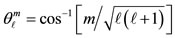 (1)
(1)
In the case of the many-body problem, however, it seems that both the angles θ and φ are specified as a result of the restrictions imposed on each particle from the neighbouring particles. When all  particles for a certain ℓ value are considered simultaneously, it seems that only one value of φ is permissible for each m value. These angles, as we rigorously show shortly, are related to the regular and semi-regular polyhedra [8].
In Figure 1 the quantization of directions for  and all associated m values
 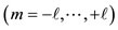 is shown in relation to the cubic-octahedral symmetry in two rows. The first row refers to
  values of m, while the second row refers to ℓ values of m with respect to an octahedron, a cube (hexahedron), or a cube-octahedron. The choice of polyhedron each time is made for reasons of clarity, while the z-axis has the same direction. The vectors ℓ forming the appropriate angles pass through char acteristic points of the polyhedra employed marked with a solid circle •. Specifically, these points for
  are
are
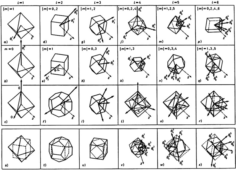
Figure 1. Orbital angular momentum (ℓ) quantization of direction for  and
and  in relation to the cube-octahedral symmetry. The vectors ℓ form accurately with the z-axis the angle
  of Eq.1. In row 3 the ℓ vectors for all m of each
  value are shown, while in rows 1 and 2 the same vectors are shown in two groups with
  and
and  values of m, respectively. In all parts of Figures 1(a)-(r) the z-axis has the same direction and all polyhedra shown are oriented with respect to the octahedron of Figure 1(a). The vectors ℓ pass through characteristic points of the polyhedra which are marked with a solid circle •, as explained in the text. Figures 1(v), (w), and (x) show an equivalent representation of ℓ vectors shown in Figures 1(k), (n), and (q), respectively and, in addition, two more ℓ vectors (shown with broken lines) already present in Figures l(j), (m), and (p). Figures 1(s)-(u) show the relationships among the polyhedra of the (o) group.
the vertices of an octahedron for both sets of m values (Figures 1(a) and (b)); for  the vertices and the shown golden section point of a cube (Figures 1(d) and (e)), respectively); for
  the middles of the edges of a cube-octahedron for both sets of m (Figures 1(g), (h)); for
  the vertices of an octahedron (Figure 1(j)) and the vertices of a cub-octahedron (Figure 1(k)); for
  the middle points of the shown line segments of an octahedron (Figure 1(m)) and of a cube-octahedron (Figure 1(n)); and for ℓ = 6 the third of the shown line segments of a cube (Figure 1(p)) and the middle points of the shown line segments of a cub-octahedron (Figure 1(q)) [8].
There is an important feature of ℓ vectors. When , the ℓ vectors of both rows of m (i.e., row 1 and row 2 in Figure 1) transform into each other by using a single transformation of the cube-octahedron symmetry group. But as one can see in Figure 1 when
 , the ℓ vectors transform into each other again by a single operation of the cubeoctahedral symmetrygroup but by a different operation for each row of m.
We have demonstrated above that the degenerate states of the same  value for the cases
  have a rotational invariance of Orbital Angular Momentum Quantization of Direction which splits into two sets of m, i.e., one referring to row 1 with
  values of m and another referring to row 2 with ℓ values of m.
In general, we may argue that the Orbital Angular Momentum Quantization of Direction implies the existence of a fundamental symmetry in nature which could be used as a basis of a physical theory of the structure of matter.
For more details see [8].
2.2. Spin and Total Angular Momentum
In this section the quantization of spin (s) and total (j) angular momenta, in relation to the geometry of regular and semi-regular polyhedra, is presented. That is, in relation to the same polyhedra employed earlier to demonstrate the quantization of the orbital angular momentum (ℓ). These polyhedra are shown in Figure 2 and are considered superimposed on each other in such a way that they have a common center, a common z-axis, and the most symmetric relative orientation to each other.
In Figure 3 the quantization of direction of the orbital (ℓ), spin (s), and total (j) angular momenta is shown in parts a), b), and c), respectively, where their relative magnitudes are also shown for ,
,  , and
, and . Apparently, the direction of each is unspecified in the polar angle φ, but it is specified in the azimuthal angle θ according to the relationship of Eq.2
 (2)
(2)
where α stands for ℓ, or s, or j and mα ιs the corresponding z-component.
In Figure 2 the geometry of quantization of the orbital angular momentum is shown for the cases  for all m, and
  for
for .
.
The quantization of direction of the spin, according to Eq.2, is given by the angles
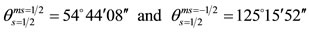 (3)
(3)
These two angles are identical to characteristic angles of the cube-octahedron (Figure 2(c)). The points A, B, C are the middles of the edges of the cube-octahedron. These spin angles are also characteristic angles of the hexa-hedron, dodeca-hedron, octa-hedron and all other polyhedra of Figure 2 because of their interrelationships shown in Figures 2(e) and (f).
The geometry of the quantization of the total angular momentum is demonstrated in Figures 2(a)-(d). For example consider ,
,  ,
,  illustrated in Figure 2(c). Eq.2 now gives
 (4)
(4)
Both vectors ℓ and s go through the middle of edges of the cube-octa-hedron (the number 1 in 16-8 stands for the middle of the edge). Applying the parallelogram rule to these vectors, we find that the resultant vector has a magnitude  and a projection on the z-axis
 , and forms an angle
  with the z-axis. That is, this resultant vector is identical to. J = ℓ + s with
  and
and .
.
Other cases examined are apparent in Figures 2(a)-(d). For more details see [9].
3. APPLICATIONS OF SYMMETRIES TO QUANTUM MECHANICS
3.1. Symmetry Description of the Independent Particle Model (IPM)
In Figure 4(a) in relation of an octahedron, the quantization of the direction of the orbital angular momentum for  is given. All expected directions are axes of symmetry passing through pairs of two opposite vertices of the octahedron, while in Figure 4(b) the quantization of direction for the spin
  are given in relation to the same polyhedron. The two directions of spin shown pass through the middles of two opposite edges of a cub-octahedron. In Figures 4(c) and (d) the total angular momentum j for
  and
and ,
, 
 , respectively, are derived by applying the parallelogram rule to the orbital angular momentum of Figure 4(a) and to the spin of Figure 4(b). In Figure 4(e),
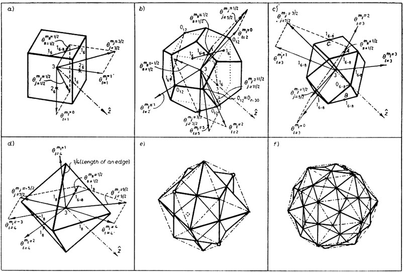
Figure 2. Equilibrium (Leech) polyhedra for the demonstration of the quantization of orbital, intrinsic, and total angular momenta. The numbers 0, 1, 2, 3 stand for the vertex, the middle of an edge, the center of a face, and the center of a polyhedron, respectively. The prefixes 6, 8, 6-8, 12, and r-30 refer to a hexa-hedron (cube) (part a), an octa-hedron (part d), a cube-octahedron (part c), a dodeca-hedron (part b) (where an inscribed cube marked with dotted lines is shown as well), and a rhombic triaconta-hedron, respectively. The symbol  stands for an orbital-angular-momentum vector ℓ having a projection mℓ on the z-axis, which is common for all polyhedra. All the θ vectors shown correspond to the quantization of direction when ℓ is a constant of the motion. The symbol
  stands for a spin vector s having a projection ms on the z-axis. When the parallelogram rule is applied to add a
  vector and another
  vector, for the cases shown, the correct total-angular momentum vector j results (having the correct projection mj on the z-axis) marked as
 . Part e): Interconnections among a tetra-hedron (only vertices are shown marked with o), a hexa-hedron, an octa-hedron, a cube-octahedron (dot-dashed lines) and a rhombic dodecahedron. Part f): Interconnection among a dodeca-hedron, an icosa-hodron, an icosi-dodeca-hedron and a rhombic triaconta-hedron (dot-dashed line).
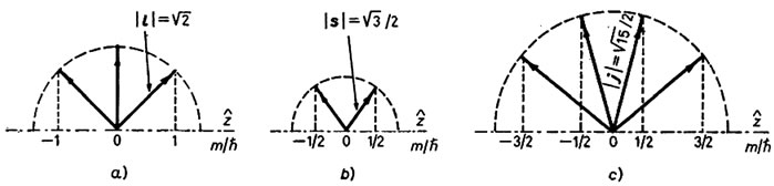
Figure 3. Relationship between the magnitudes of orbital angular momentum a), spin b), and total angular momentum c), and their z-components.
however, the case ,
,  is presented, where neither ℓ nor s come from Figures 4(a) and (b). In Figures 4(c)-(e) j, and not ℓ or s, is the constant of the motion, thus the ℓ and s do not necessarily maintain the same directions in space as in Figures 4(a) and (b). The j in Figure 4(e) is determined in relation to the j of Figures 4(c) and (d) according to the law of addition of angular momenta, as will become apparent in a short time. As shown, this is the only case in which j does not pass through the middle of the relevant line segment. For simplicity in Figures 4(c)-(e) the cases of j with negative mj are omitted. However, j (with +mj) equals –j (with –mj).
So far, in Figures 4(c)-(e), we have determined in relation to an octahedron, the total angular momenta for individual particles which have pairs of j and mj values appropriate for an assignment to p states. This, of course, guarantees only that the angles of j with the z-axis, i.e. the angles  are correct and does not guarantee that the vectors j themselves are those expected by the IPM for p states, which is the purpose of this section. The vectors j of Figures 4(c)-(e) must have, in addition, the appropriate relative orientation in such a way that, when the j of two individual particles (e.g. j1 and j2) are coupled together, the correct total J of the system results. That is the vectors j1 and j2 must form the appropriate angle.
Figures 4(f)-(n) shows that the j vectors of Figures 4(c)-(e), in the framework of the symmetry of an octahedron, possess the appropriate relative orientations which lead to the correct coupling of the total angular momenta of two particles for all cases with ℓ = 1. Specifically, Figures 4(f) and (g) demonstrate that the j of Figures 4(c)-(e) result in the correct total J for the system of two particles with . Figures 1(h)-(l) demonstrate that these j also result in the correct J, where
 . Figures 4(m)-(n) demonstrate the same when
  and
and  as registered on each relevant part of the figure. Thus it has been found that the j vectors of Figures 1(c)-(e) are indeed the IPM j.
For more details see [10].
3.2. Applications to Nuclear Structure
3.2.1. Semi-Classical Isomorphic Shell Model
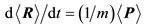
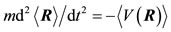
Here, we present the semiclassical part of the model, which has been used many times [11-13] in place of the quantum mechanical part of the model [14], in the spirit of the Ehrenfest theorem [15,16] (that for the average values, the laws of Classical Mechanics are valid). The vertices of the polyhedra of Figure 5 stand for the distribution of the maxima of the wave function for nucleons due to the anti-symmetric requirement of this function. The Ehrenfest theorem for the observables of position  and momentum
  takes the form (see all details in [16]).
 (5)
(5)
and
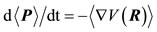 (6)
(6)
For simplicity here, the case of a spinless particle in a scalar stationary potential  is considered.
The quantity  represents a set of three time-dependent numbers
  and the point
  is the center of the wave function at the instant t. The set of those points which correspond to the various values of t constitutes the trajectory followed by the center of the wave packet.
From Eqs.5 and 6 we get
 (7)
(7)
Furthermore, it is known [16] that for special cases of force, e.g., for the harmonic oscillator potential assumed by the model, the following relationship is valid:
 , (8)
, (8)
where
 . (9)
. (9)
That is, for this potential the average of the force over the whole wave function is rigorously equal to the classical force F at the point where the center of the wave function is considered. Thus, for the special case of potential considered here, the motion of the center of the wave function precisely obeys the laws of classical mechanics [16]. Any difference between the quantum and the classical description of the nucleon motion exclusively depends on the degree that the wave function may be approximated by its center. Any such difference would contribute to deviations between the experimental data and the predictions of the semiclassical part of the model employed.
Thus, in the present semiclassical treatment the nuclear problem is reduced to that of studying the centers of the wave functions of the constituent nucleons or, in other words, of studying the average positions of these nucleons [17].
We further proceed with the help of Figure 5 which is identical to that figure employed in [11-13], where the most probable forms and average sizes of the first three proton and the first three neutron shells are presented. It is essential to mention that these average sizes solely depend on the average size of a proton, rp = 0.860 fm, and that of a neutron, rn = 0.974 fm. Each occupied vertex configuration of this figure corresponds to a quantum state configuration with definite angular momentum and energy. More details of the figure are given in its caption.
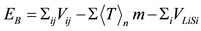
The expressions of the two-body (two Yukava) potential V employed [18], for the present semi-classical treatment, of the kinetic energy T [19], of the spin-orbit energy VLS [20], and of the binding energy EB are given in Eqs.10-14, respectively. Isospin term in Eq.14 is not
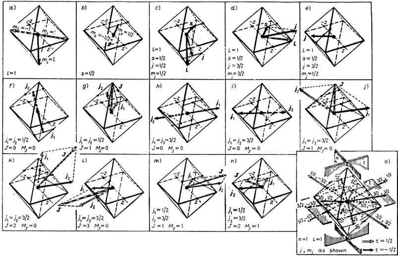
Figure 4. Octa-hedral symmetry description of the Independent Particle Model (IPM) for the 1p-shell. Each mark • stands for the middle point of the corresponding straight-line segment, while large • stands for the center of the octa-hedron. Dark arrows stand for protons and open ones for neutrons, or the opposite, but no mixed [10]. Orbital angular-momentum vectors stand for both protons and neutrons and are presented by dark-open arrows [10]. All j shown are in a relative scale; a) and b) quantisation of direction, when the orbital angular momentum ℓ or spin s are constants of the motion, respectively; c)-e) considered together: quantization of direction when the total angular momentum j is a constant of the motion; f)-n) total angular momentum J of two particles with j1 and j2 as registered on each related part; o) assignment of a set of five quantum numbers (n, ℓ, j, mj and τ) to each j vector of an IPM description of p-shells.
needed since the isospin is here taken care of by the different shell structure (forms and sizes) between proton and neutron shells, as apparent from Figure 5.
 (10)
(10)
 (11)
(11)
 (12)
(12)
 (13)
(13)
 , (14)
where
• Vij is the potential energy between a pair of nucleons i, j at a distance rij• n, ℓ, m are the quantum numbers characterizing a polyhedral vertex standing for the average position of a nucleon at the quantum state n, ℓ, m.
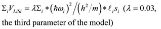
• ℓi and si stand for the orbital angular momentum quantum number ℓ and the intrinsic spin quantum number s of any nucleon i.
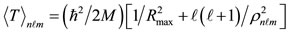
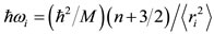
• M is the mass of a proton Mp or of a neutron Mn• Rmax is the outermost proton or neutron polyhedral radius (R) plus the relevant average nucleon radius rp for a proton and rn for a neutron, (i.e., Rmax is the radius of the nuclear volume in which protons or neutrons are confined)• ρnℓm is the distance of a nucleon average position at a quantum state (n, ℓ, m) from its orbital angular momentum at the direction nθ .
.
The parameters of the model are the following five: the two-size parameters rp and rn, the two parameters from the second term of Eq.10 (since the first term is applicable only for scattering problems), and the one parameter, λ, from Eq.12. With the help of these parameters all quantities Rmax, ρnℓm, and ћωi in Eqs.10-14 are obtainable by employing the coordinates of the nucleon
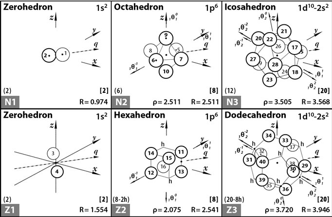
Figure 5. The space of the Isomorphic Shell Model for nuclei up to N = 20 and Z = 20. The equilibrium polyhedra in row 1 (2) stand for the most probable forms and average sizes of the first three neutron (proton) shells. The vertices of polyhedra (numbered as shown) stand for average positions of nucleons in definite quantum states (τ, n, ℓ, mℓ, s). Central axes standing for the quantization of directions of the orbital angular momentum are labelled as  and pass through the points marked by small solid circles •. At the bottom-left of each block the numbering of this polyhedron proceeded by the letter Z (N) for protons (neutrons) is given. Over this the number of polyhedral vertices and the number of possible unoccupied vertices (holes, h) are also given. At the bottom-right of each block the radius of polyhedron is listed. Over this the cumulative number of vertices of all previous polyhedra and of this polyhedron is also given. Finally, at the bottom-center of each block the distance ρnℓm of the nucleon average position nℓm from the relevant axis
  is given.
average positions derived by the information given in Figure 5.
In Table 1 the results of applying the present version of the model for 4He, 12C, 16O, and 40Ca, together with corresponding experimental energies are given. The good comparisons between model predictions and experimental energies are apparent. Here, calculations of radii are not presented. Such predictions for more nuclei are given in the next section with a full quantum mechanical description of the Isomorphic Shell Model. In the framework of predictions of radii, results are identical for both versions of the model.
Further interesting applications of this version of the model on nuclear structure and reactions are included in Refs. [11-13] and [21,22], respectively.
3.2.2. Quantum Mechanical Isomorphic Shell Model
As is well known the constituent of a nucleus are protons and neutrons which all are fermions, thus their total wave function is anti-symmetric. The locations of maxima of such a wave function on a sphere (like the spherical shape of a complete nuclear shell) are identical to those expected if a repulsive force (of unknown nature) is acting among the constituent fermions (protons and neutrons) [23]. For stability these maxima, under the aforementioned repulsive force, should be in equilibrium.
This problem of equilibria of repulsive particles on a sphere was solved by John Leech in1957 [24]. Such equilibria are obtained only for specific number of particles and are related either to the number of vertices, or to the number of middles of edges, or to the number of middles of faces, or to combinations of numbers of these categories of a regular or semi-regular polyhedron [14].
Such equilibria lead to polyhedral most probable forms which, taken in specific sequence, are presented in Figure 6 and are related to specific nuclear shells and sub-shells. If further, nucleons of finite sizes are considered (specifically, rp = 0.860 fm and rn = 0.974 fm, which constitute the only size parameters of the model) the average size R of the aforementioned polyhedral
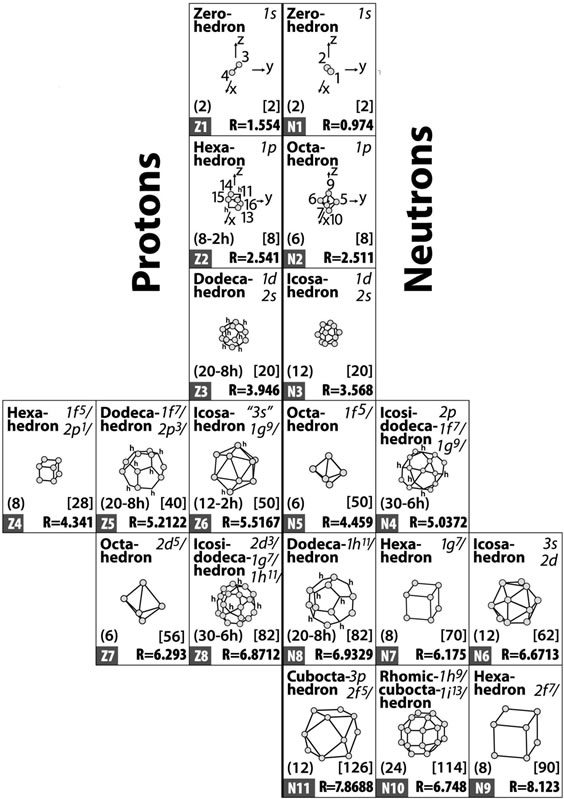
Figure 6. Most probable forms and average sizes of nuclear shells and sub-shells for nuclei up to Z = 82 and N = 126. Other notations are as in the caption of Figure 5.
shells and subshells are obtained. They are those written at the bottom of each block of the figure.
Apparently, the polyhedra of Figure 6 present the most probable forms and average sizes of nuclear shells and sub-shells and at the same time are the same polyhedra as the ones of Figures 1-4, i.e., they are again the regular and semi-regular polyhedra. That is, these polyhedra inherently possess quantum mechanics and at the same time they are those polyhedra possessing equilibrium of forces when repulsive particles (or equivalently fermion average positions) fill up their vertices, or middles of edges, or middles of faces.
Some more comments should be made concerning the polyhedra of Figure 6 and the major models of nuclear structure, i.e., the Shell Model and the Collective Model.
The first model assumes independent particle motion of the constituent particles of a nucleus, which is equivalent to assuming zero forces among these particles in a strong field of strong interactions like a nucleus. In addition, this model it does not give the range of applicability of the assumption and how one can understand the difference of stability (if any) between the magic numbers
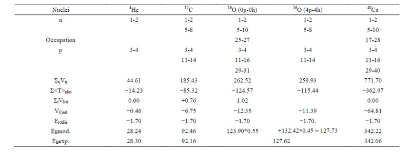
Table 1. Binding energies in MeV according to semi-classical isomorphic shell model.
and the other (about 300) stable nuclei spread in the chart of the nuclides. Moreover, the shell model tries to explain the magic numbers by arbitrarily assuming a strong spin orbit interaction valid only for magic numbers, which is not a necessary assumption for other models (like the present one) to explain these numbers.
The second model assumes strong interaction among the constituent particles of a nucleus leading to an average form of the nucleus which can possess collective motion. This assumption apparently contradicts the shell model assumption of zero forces among the constituent particles of a nucleus. The model has many successes through out the periodic table of the elements. However, it cannot predict the moment of inertia of the resulting rotational spectra at the same time. This moment of inertia is empirically derived each time from the rotational spectrum offered by relevant experiments.
Apparently, these two models were milestones at the time when they appeared. Without these two basic models we could not have reached the present level of understanding about the nucleus. After so many years since their appearance, there is an effort to try to go beyond them.
The Isomorphic Shell Model takes advantage of the equilibrium polyhedra to explain the magic numbers without assuming strong spin orbit interaction and at the same time provides the average structure of a nucleus via the average nucleon positions of the constituent nucleons. Thus, it provides the necessary moment of inertia as the moment of inertia of a specific part of the nucleus which rotates around an axis perpendicular to a symmetry axis of this rotating part. Also, the equilibrium of forces obtained when an equilibrium polyhedron is filled is equivalent to the zero forces assumed by the shell model. However, this equilibrium of forces happens not only for magic numbers, but at any time an equilibrium polyhedron is filled up, a fact which explains stable nuclei throughout the periodic chart of nuclides.
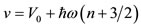
In applying the quantum isomorphic shell model a central potential of the following form is applied for the nucleons of each proton or neutron shell (and not for all nucleons in a nucleus):
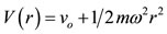 (15)
(15)
where v0 and ω are different parameters for each proton or neutron shell. Due to the two assumptions below, however, the final number of parameters is substantially reduced.
1) The , for each shell, is determined [20] according to Eq.16,
 (16)
(16)
where  is the average size of a specific proton or neutron shell which remains constant for all nuclei. All these sizes of polyhedra are given in Figure 6. The only parameters necessary in determining these sizes are the two size parameters rp and rn, as explained earlier.
2) The parameter of the depth of the potential for each proton or neutron shell is determined according to Eq.17
 or
or
 (17)
(17)
This assumption implies that all nucleons in a nucleus are equally bound in their own potentials (excluding Coulomb and spin-orbit interactions).
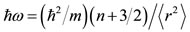
It is apparent from Eq.17 that, since according to the previous assumption a) all ћω are already determined as above by applying Eq.16 with respect only to the two size parameters rp and rn, the depth vi of the potential for each shell i can be defined with the knowledge of only one additional parameter V0 (This is the third universal parameter of the present model equal to 40.268 MeV.)
Solving Schroedinger’s equation for the potential of Eq.15, the following general equation for the wave function is obtained [20]:
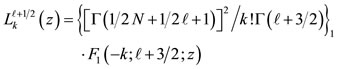 , (18)
where 
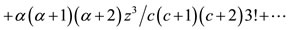 , with
 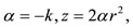 and
and . The series terminates with the term
  and the various quantum numbers involved are
 ,
,  and
and  [20].
[20].
The explicit forms of equations of the wave functions for a harmonic oscillator potential derived from the recursion formula Eq.18 can be found in [14] for all wave functions of nuclei up to Z = 126 and N = 184.
Due to the fact that in the model ћω is different for the different shells, the wave functions with the same orbital angular momentum quantum number ℓ are not orthogonal. For these wave functions Gram-Smidth’s technique is applied [25]. In [14] some relevant guide equations to facilitate this orthogonalization are given.
1) Binding Energies
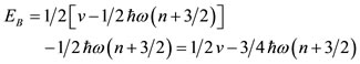
The binding energy for each quantum state in a harmonic oscillator potential is given by Eq.19:
 (19)
(19)
In Eq.19 all ћω come from Eq.16 (with respect to the only two size parameters rp and rn) and all potential depths v come from Eq.17 (with respect to the only one additional potential parameter V0). Thus, EB from Eq.19 is determined with respect to only 3 universal parameters.
Now, since the nuclear problem basically refers to two-body forces, in order to avoid the double counting, the potential portion of the second part of Eq.19 should be divided by two. Furthermore, since according to the Virial theorem half of the quantity  is potential energy and half is kinetic energy, Eq.19 takes the form of Eq.20
 (20)
(20)
Given that the potential v, according to Eq.17, is
 , (21)
the final expression of binding energy for each proton or neutron state takes the form of Eq.22.
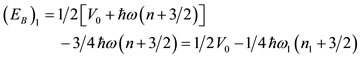 . (22)
The index 1 in Eq.22 refers to all states where the orbital angular momentum quantum number ℓ appears for the first time.
However, for a second, a third and a fourth appearance of a state with the same ℓ, in the place of the quantity  in Eq.22 we should take the corresponding quantity due to the necessary orthogonalization by using Eqs.9-11 of [14]
Finally, the total binding energy of a nucleus in the model is given by Eq.23
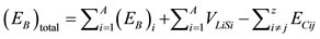 , (23)
where the spin-orbit term is given [20] by Eq.24
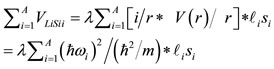 , (24)
with λ = 0.03 (This is the fourth and the last universal parameter of the present version) and the Coulomb term is given by Eq.25:
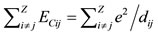 . (25)
The distance dij between any two proton average positions in Figure 6 is calculated from the coordinates of the proton polyhedral vertices (standing for the proton average positions) in this figure (see section 2.2 of [14]).
As in the former section, an extra term in Eq.23 due to isospin is not needed since the isospin is here taken care of by the different average shell structure between protons and neutrons as apparent from Figure 6.
2) Mean Radii
Due to the way the wave functions have been correlated with the size of nuclear shells via Eq.16, average radii can be calculated by using simple formulas, as seen below.
Average charge radius:
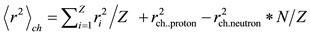 , (26)
where rch.proton = rp = 0.86 fm and rch.neutron = 0.34 fm [7].
Average neutron radius:
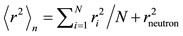 , (27)
where .
.
Average mass radius:
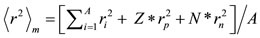 . (28)
All values of ri needed are included in Figure 6 (see right corner at the bottom of each block).
In Table 2 the binding energies of 40Ca, 48Ca, 54Fe, 90Zr, 108Sn, 114Te, 142Nd, and 208Pb. are listed from [14]. Also for the same nuclei the average charge, neutron, and mass radii are listed again from [14]. For both energies and radii available experimental values are given for comparison. The very good agreements between predictions and experimental values are apparent.
3.2.3. Other Applications
Besides the above given applications of the Isomorphic Shell Model, it is interesting to mention its application to super-heavy nuclei [26], to neutron nuclei [27], to exotic nuclei [28], and its extension to atomic clusters [29], when the constituents atoms have half integer spin and thus can be considered as atomic fermions. Again in these applications the dominant part is the relationship between Symmetry of regular and quasi-regular polyhedra and Quantum Mechanics.
For valuable information concerning geometry, the books [30,31] are very instructive.
4. CONCLUSIONS
In the present work, the regular and semi-regular polyhedra were employed to derive the relationship between their symmetries and quantum mechanics. Particularly, we showed that the symmetries of these polyhedra inherently possess (on the level of identity) the quantization of ℓ, s, and j expected from Quantum Mechanics for central forces. This is a unique property of the present model in comparison with the other models of the nucleus involving polyhedra to explain the magic numbers and other nuclear properties. No relationship of their polyhedra with Quantum Mechanics has been reported. This unique property of the present work to identically connect the symmetry of the regular and semi-regular polyhedra with Quantum Mechanics permits one to assign quantum states at the vertices of these polyhedra considered as the average positions of neutrons and protons in the way explained in the text.
Furthermore, an important feature of the polyhedra employed in the present work (i.e., the regular and semiregular polyhedra) is that they possess the equilibrium property. That is, when repulsive particles (as implied by the Pauli principle for fermions) are assigned at their vertices, standing as their average positions, these particles are at equilibrium whatever the law of force between them may be. In addition, if two sets of fermions are assumed on the same sphere (as neutrons and protons), not only the particles of each set, but also the particles of both sets should be at equilibrium. This equilibrium should be conserved when more polyhedral shells are considered, which implies that the polyhedra should be concentric and in the most symmetric arrangement among themselves. This property of equilibrium of forces is practically equivalent to the assumption of the Shell Model of the nucleus that each nucleon acts as if it is under a zero force.
This equilibrium property leads to the most probable forms of nuclear shells. As mentioned in the introduction, neutrons and protons are not considered as point particles, but as particles with finite size, which have been established from particle physics. The consideration of nucleons with finite size leads to the average size of the nuclear shells and thus of all nuclei. These average positions for the nucleons participating in a collective nuclear rotation form an average shape whose symmetries permit the evaluation of moments of inertia and thus of the energies of the expected rotational bands for this nucleus. This is the way the present work is associated with the Collective Model of the nucleus.
However, there is an important difference between the Collective Model and the present model. In the former, it is assumed that the rotating nucleons strongly interact with each other (like in solid state physics) and form the rotating shape necessary for the rotational band. However, the Collective Model still cannot predict the moment of inertia. The present model does not need this additional assumption. It can predict the moment of inertia and the rotational band based on the average positions of rotating nucleons derived as above.
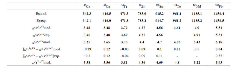
Table 2. Total binding energies in MeV, average charge, neutron, point neutron-proton, and mass radii.in fm [14].
A further strong support of this work is provided by its application to specific nuclear properties. First, the ћω values are estimated in both the semi-classical and pure quantum mechanical treatment of nuclei. Specifically, in Table 1 the nuclei 4He 12C, 16O and 40Ca are treated semi-classically and their binding energies have been estimated with a maximum deviation between predicted and experimental values of 0.30 MeV. In Table 2 the nuclei 40Ca, 48Ca, 54Fe, 90Zr, 108Sn, 114Te, 142Nd, and 208Pb are treated purely quantum mechanically. Properties examined there are the binding energies and radii. The maximum deviation between predicted and experimental values of binding energies is 0.5 MeV. For the average values of charge radii, predicted and experimental values are identical, with the only exception for 54Fe where the difference is 0.03 fm. For the difference between neutron and proton average radii in the same table the deviation is 0.01 fm, except for 208Pb, where the deviation is 0.09 fm and is considered significant. For the average neutron radii, there are no experimental values for comparison.
Other applications of the present model are given elsewhere [14]. Hence, a very strong connection between Polyhedral Symmetry and Quantum Mechanics is provided throughout this work.
Perhaps it is interesting to finish with Albert Einstein’s words: Geometry is always the solution. The question is which geometry each time.
REFERENCES
- Pauling, L. (1990) Regularities in the sequences of the number of nucleons in the revolving clusters for the ground-state energy bands of the even-even nuclei with neutron number equal to or greater than 126. Proceedings of the National Academy of Science USA, 87, 4435-4438, and references therein. http://dx.doi.org/10.1073/pnas.87.12.4435
- Cook, N.D. (1994) Nuclear binding energies in lattice models. Journal of Physics G (Nuclear and Particle Physics), 20, 1907-1917 and references therein.
- Rae, W.D.M. and Zhang, J. (1994) Triangular alpha cluster geometries and harmonic oscillator shell structure. Modern Physics Letters A, 9, 599-607 and references therein. http://dx.doi.org/10.1142/S021773239400383X
- Robson, D. (1978) Many-body interactions from quark exchanges and the tetrahedral crystal structure of nuclei. Nuclear Physics A, 308, 381-428 and references therein. http://dx.doi.org/10.1016/0375-9474(78)90558-4
- Naher, U., Zimmermann, U. and Martin, T.P., (1993) Geometrical shell structure of clusters. Journal of Chemical Physics, 99, 2256-2260. http://dx.doi.org/10.1063/1.465235
- Hecht, L. (1988) The geometrical basis for the periodicity of the elements.
- White, (1987) New hypothesis shows geometry of atomic nucleus. Executive Intelligence Review, 14, 18.
- Anagnostatos, G.S., Giapitzakis, J. and Kyritsis, A. (1981) Rotational invariance of orbital-angular-momentum quantization of direction for degenerate states. Lettere Nuovo Cimento, 32, 332-335. http://dx.doi.org/10.1007/BF02745301
- Anagnostatos, G.S. (1980) The geometry of the quantization of angular momentum (ℓ, s, j) in fields of central symmetry. Lettere Nuovo Cimento, 28, 573-576. http://dx.doi.org/10.1007/BF02776343
- Anagnostatos, G.S. (1980) Symmetry description of the independent particle model. Lettere Nuovo Cimento, 29, 188-192. http://dx.doi.org/10.1007/BF02743377
- Anagnostatos, G.S., Ginis, P. and Giapitzakis, J. (1998) α-Planar states in 28Si”. Physical Review C, 58, 3305- 3315. http://dx.doi.org/10.1103/PhysRevC.58.3305
- Kakanis, P.K. and Anagnostatos, G.S. (1996) Persisting α-planar structure in 20Ne. Physical Review C, 54, 2996- 3013. http://dx.doi.org/10.1103/PhysRevC.54.2996
- Anagnostatos, G.S. (1999) Alpha-chain states in 12C”. Physical Review C, 51, 152-159. http://dx.doi.org/10.1103/PhysRevC.51.152
- Anagnostatos, G.S. (2013) Quantum isomorphic shell model: Multi harmonic shell clustering in nuclei. Journal of Modern Physics, 4, 54-65. http://dx.doi.org/10.4236/jmp.2013.45B011
- Merzbacher, E. (1961) Quantum mechanics. John Wiley and Sons Ltd., New York, p. 42.
- Cohen-Tannoudji, C., Diu, B. and Laloe, F. (1977) Quantum mechanics. John Wiley & Sons Ltd., New York, p. 240.
- Anagnostatos, G.S., Antonov, A.N., Ginis, P., et. al. (1998) Nucleon momentum and density distributions in 4He considering internal rotation. Physical Review C, 58, 2115- 2119. http://dx.doi.org/10.1103/PhysRevC.58.2115
- Anagnostatos, G.S. and Panos C.N. (1982) Effective twonucleon potential for high-energy heavy-ion collisions. Physical Review C, 26, 260-264. http://dx.doi.org/10.1103/PhysRevC.26.260
- Panos, C.N. and Anagnostatos, G.S. (1982) Comments on a relation between average kinetic energy and meansquare radius in nuclei. Journal of Physics G: Nuclear Physics, 8, 1651-1658. http://dx.doi.org/10.1088/0305-4616/8/12/007
- Hornyak, W.F. (1975) Nuclear structure. Academic, New York, pp. 13, 240, 237.
- Anagnostatos, G.S. (1989) Classical equations-of-motion model for high-energy heavy-ion collisions. Physical Review C, 39, 877-883.
- Anagnostatos, G.S. and Panos, C.N. (1990) Semiclassical simulation of finite nuclei. Physical Review C, 42, 961- 965. http://dx.doi.org/10.1103/PhysRevC.42.961
- Sherwin, C.W. (1959) Introduction to quantum mechanics. Holt, Rinehart and Winston, New York, p. 205.
- Leech, J. (1957) Equilibrium of sets of particles on a sphere. Mathematical Gazette, 41, 81-90. http://dx.doi.org/10.2307/3610579
- Vergados, J.D. (1970) Mathematical methods in physics. Akourastos Giannis.
- Anagnostatos, G.S. (2008) A new look at super-heavy nuclei. International Journal of Modern Physics B, 22, 4511- 4523. http://dx.doi.org/10.1142/S0217979208050267
- Anagnostatos, G.S. (2008) On the possible stability of tetraneutrons and hexaneutrons. International Journal of Modern Physics E, 17, 1557-1575. http://dx.doi.org/10.1142/S0218301308010568
- Paschalis, S. and Anagnostatos, G.S. (2013) Ground state of 4-7H considered internal collective rotation. Journal of Modern Physics, 4, 66-77. http://dx.doi.org/10.4236/jmp.2013.45B012
- Anagnostatos, G.S. (1991) Fermion/boson classification in micro-clusters. Physics Letters A, 157, 65-72. http://dx.doi.org/10.1016/0375-9601(91)90410-A
- Cundy, H.M. and Rollett (1961) Mathematical models. 2nd Edition, Oxford University Press, Oxford.
- Coxeter, H.S.M. (1963) Regular polytopes. 2nd Edition, The Mcmillan Company, New York.