Engineering
Vol. 4 No. 1 (2012) , Article ID: 17096 , 13 pages DOI:10.4236/eng.2012.41005
On the Dynamic Behavior of Town Gas Pipelines
Department of Production Engineering and Machine Design, Faculty of Engineering, Port-Said University, Port-Said, Arab Republic of Egypt (ARE)
Email: dr_eng_aly@hotmail.com
Received August 7, 2011; revised October 7, 2011; accepted October 20, 2011
Keywords: Piping Vibrations; Modal Analysis; Dynamic Susceptibility; Time History; Response Spectrum; Earthquakes
ABSTRACT
Pipelines have been acknowledged as the most reliable, economic and efficient means for the transportation of gas and other commercial fluids such as oil and water. The designation of pipeline system as “lifelines” signifies that their operation is essential in maintaining the public safety and well being. A pipeline transmission system is a linear system which traverses a large geographical area, and soil conditions thus, is susceptible to a wide variety of hazards. This paper is concerned with the dynamic behavior of buried town gas pipelines. A computer model with a finite number of nodes is created to simulate the behavior of the real gas pipeline. The dynamic susceptibility method is applied for twenty mode shapes of this model, which utilizes the stress per velocity method and is an incisive analytical tool for screening the vibration modes of the system. It can be readily identified, which modes, if excited, could potentially cause large dynamic stresses. This paper discusses also two of the piping dynamic analyses, namely the effect of the response spectrum of an earthquake and the time history analysis of a truck crosses the pipeline.
1. Introduction & Literature Review
Gas distribution systems are one of six broad categories of infrastructure grouped under the heading “lifelines”. Together with electric power, water and liquid fuels, telecommunications, transportation and wastewater facilities, they provide the basic services and resources upon which modern communities have come to rely, particularly in the urban context. Disruption of these lifelines through damage can therefore have a devastating impact, threatening life in the short term and a region’s economic and social stability in the long term. Pipeline system consists of buried and above ground pipelines, above ground facilities such as pumping stations, storage tanks and miscellaneous terminal facilities. However the term pipeline in general implies a relatively large pipe spanning a long distance.
[1] obtained the amplitude and frequency of vibration by testing the vibration signals from the compressor pipeline, used ANSYS software for the calculation, and reduced the amplitude of vibration by adding supports to alter the frequency of the pipeline. [2] presented numerical simulation of pipeline system using finite element method (FEM) to calculate for the modal analysis, consonance dynamic and steady-state analysis, and found reasonable pipeline structure parameters on the basis of analyzing dynamic vibration performance of pipelines for reducing vibration and enhancing the production security. [3] analyzed the vibration of reciprocating compressor gas pipeline as a frequent problem which always affected normally running condition of the equipment. [4] applied the method of vibration analysis, probed into the vibration of gas pipeline, analyzed the vibration reason, and put forward the correspondingly damping measures. For analyzing the vibration in gas transmission line system by [5], the change of flow parameters was analyzed first according to the unsteady state flow of the gas in pipeline system and then the acting force of the gas flow on pipeline system was determined, and based on this and in the light of the borne pressure in pipeline system, the vibration was analyzed by using intensive quality method and finally the calculation example was given out.
[6] analyzed the vibration induced by fluid pulsation for a section of gas pipeline, used the FEM method, and considered the influence of the factors such as the complex restraints of the pipeline system, the components of the pipeline system, the steel structure etc. on the vibration of the pipeline system. [7] used the FEM method to calculate the support stiffness, by varying the support points and the stiffness of the pipeline system, the calculation process was repeated until the best modified version of decrease in vibrations was obtained. [8] analyzed the dynamic response induced by seism for a section of gas pipeline system, with finite element modeling, considering the influence of the complex supports, hangers, devices and elbows of the pipeline system, the system modality induced by 3-D Elcentro seism, the response amplitudes of the system displacements and rotations, and the response coefficient of the system modality induced by seism were calculated. The results showed seism had big effect on the performance of the pipeline system, which should be considered when pipeline design was made. The measures were proposed to improve the anti-seismic property of the pipeline system.
The liquefied soil will do great damage to buried pipeline during an earthquake. It causes a floating force and leads to floating response that is a dynamic process varying with time. [9] simplified the underground pipeline in liquefied soil under the action of seismic loading as a model of a simple beam with elastic supports on two ends and considering the interaction of buried pipelinesoil and fluid-structures, the authors use the mode superposition method to analyze the dynamic seismic response. The influence of various pipeline and liquefied soil parameters on floating response was discussed. The dynamic floating displacement of pipeline and how it varies with the parameters of flow velocity, fluid pressure, fluid density, axial force of pipe section, damping of pipe material, the specific gravity and relative elastic coefficient of liquefied soil and the amplitude of seismic acceleration was calculated and analyzed. The results indicate that the dynamic seismic response analysis method is successful and meaningful. [10] considered Newmark and Hall’s theoretical model to analyze the laid pipeline. It was found out that the stiffness of the pipeline is the major aspect in this seismic zone for the safe operation of the pipeline system. The stiffness of the pipeline depends on various physical parameters of the pipe such as diameter, thickness and material property.
In addition to the modal frequencies and mode shapes, the pipeline modal analysis includes new outputs called dynamic stresses and dynamic susceptibility. These new outputs are based on modal analysis method by a PC computer program. The dynamic susceptibility method is essentially a post processor to fully exploit the modal analysis results from the piping system [11,12]. The pipeline designer does not have either the specific requirements, or the analytical tools and technical references which are typically available for other plant equipment such as rotating machinery. Piping vibration problems only become apparent at the time of commissioning and early operation, after a fatigue failure or degradation of pipe supports.
The underlying theoretical basis for the Stress/Velocity method is a deceptively straightforward but universally-applicable relationship between kinetic energy and potential (elastic) energy for vibrating systems. Stated simply, for vibration at a system natural frequency, the kinetic energy at maximum velocity and zero displacement must then be stored as elastic (strain) energy at maximum displacement and zero velocity [13]. Since the strain energy and kinetic energy are respectively proportional to the squares of stress and velocity, it follows that dynamic stress, σ will be proportional to vibration velocity, v [14]. For idealized straight-beam systems, consisting of thin-walled pipe and with no contents, insulation or concentrated mass, the ratio σ/v is dependent primarily upon material properties (density ρ and modulus of elasticity E), and is remarkably independent of system-specific dimensions, natural-mode number and vibration frequency. For real continuous systems of course, the kinetic and potential energies are distributed over the structure in accordance with the respective mode shapes [15]. Provided the spatial distributions are sufficiently similar, i.e. harmonic functions. Many programs have been developed to assure reliability and plant safety with respect to vibration while minimizing cost and delay time [16].
At the design stage, the dynamic susceptibility method allows the designer to quickly identify and correct features that could lead to large dynamic stresses at frequencies likely to be excited. The method provides a quick and incisive support to efforts of observation, measurement, assessment, diagnosis, and correction. Furthermore, it reveals which features of the system layout and support are responsible for the susceptibility to large dynamic stresses. The dynamic stresses are the dynamic bending stresses associated with vibration in a natural mode [15]. The dynamic susceptibility for any mode is the ratio of the maximum alternating bending stress to the maximum vibration velocity. This susceptibility ratio provides an indicator of the susceptibility of the system to large dynamic stresses. The Stress/Velocity method for screening piping system modes was developed and presented to the attention of SST Systems company by Dr. R. T. Hartlen of Plant Equipment Dynamics Inc. [17].
Buried gas pipelines structures, when subjected to loads or displacements, behave dynamically. If the loads or displacements are applied very slowly then the inertia forces can be neglected and a static load analysis can be justified [18]. Hence, dynamic analysis is a simple extension of static analysis. Two types of vibration excitation are considered in this work, namely the influence of an earthquake through its response spectrum and the time history analysis of a truck, which crosses the gas pipeline.
2. Underlying Fundamental Basis of the Method
2.1. Kinetic Energy and Potential Energy; Vibration Velocity and Dynamic Stresses
The underlying theoretical basis for the Stress/Velocity method is a deceptively straightforward but universallyapplicable relationship between kinetic energy and potential (elastic) energy for vibrating systems. Stated simply, for vibration at a system natural frequency, the kinetic energy at maximum velocity and zero displacement must then be stored as elastic (strain) energy at maximum displacement and zero velocity. Since the strain energy and kinetic energy are respectively proportional to the squares of stress and velocity, it follows that dynamic stress, ó, will be proportional to vibration velocity, v. For idealized straight-beam systems, consisting of thin-walled pipe and with no contents, insulation or concentrated mass, the ratio ó/v is dependent primarily upon material properties (density ρ and modulus E), and is remarkably independent of system-specific dimensions, natural-mode number and vibration frequency.
For real continuous systems of course, the kinetic and potential energies are distributed over the structure in accordance with the respective modes shapes. However, integrated over the structure, the underlying energyequality holds true. Provided the spatial distributions are sufficiently similar, i.e. harmonic functions, the rms or maximum stress will still be directly related to the rms or maximum vibration velocity.
2.2. The “Screening” Approach
As stated above, for idealized pure beam systems the stress-velocity ratio will depend primarily upon material properties. For real systems, the spatial patterns of the mode shapes will depart from the idealized harmonic functions, and the stress-velocity ratios accordingly increase above the theoretical minimum or baseline value. System details causing the ratios to increase would include the three-dimensional layout, large unsupported masses, high-density contents in thin-walled pipe, susceptible branch connections, changes of cross section etc. The more “unfavorable” is the system layout and details, the larger will be the ó/v ratios for some modes.
Thus, the general susceptibility of a system to large dynamic stresses can be assessed by determining the extent to which the ó/v ratios for any mode exceed the baseline range. Furthermore, by determining which particular modes have the high ratios, and whether these modes are known or likely to be excited, the at-risk vibration frequencies and mode shapes are identified for further assessment and attention. This is the basis of the Stress/Velocity method of analysis and its implementation as the “dynamic susceptibility” feature in [17].
2.3. Relation to Velocity-Based Vibration Acceptance Criteria
There are various general and application-specific acceptance criteria based upon vibration velocity as the quantity of record. Some, in order to cover the worst case scenarios, are overly conservative for many systems. Others are presented as being applicable only to the first mode of simple beams, leading to the misconception that the Stress/Velocity relationship does not apply at all to higher modes. In any case, there are real and perceived limitations on the use of screening acceptance criteria based upon a single value of vibration velocity.
The dynamic susceptibility method turns this apparent limitation into a useful analytical tool! Specifically, large Stress/Velocity ratios, well above the baseline values, are recognized as a “warning flag”. Large values indicate that some feature(s) of the system make it particularly susceptible to large dynamic stresses in specific modes.
2.4. What the Dynamic Susceptibility Method Does?
2.4.1. General Approach
The Dynamic Susceptibility method is essentially a post processor to fully exploit the modal analysis results of the system. Mode shape tables of dynamic bending stress and vibration velocity are searched for their respective maxima. Dividing the maximum stress by the maximum velocity yields the “ó/v ratio” for each mode. That ratio is the basis for assessing the susceptibility to large dynamic stresses. Larger values indicate higher susceptibility associated with specific details of the system.
2.4.2. Specific Implementation in CAEPIPE
The Stress/Velocity method has been implemented as additional analysis and output of the CAEPIPE modal analysis. The modal analysis load case now includes additional outputs and features as follows:
Dynamic Stresses: This output provides the “mode shapes” of dynamic bending stresses, tabulated along with the conventional mode shape of vibration magnitude.
Dynamic Susceptibility: This output is a table of s/v ratios, in psi/ips, mode by mode, in rank order of decreasing magnitude. In addition to modal frequencies and s/v ratios, the table also includes the node locations of the maxima of vibration amplitude and bending stresses.
With the dynamic susceptibility output selected, the animated graphic display of the vibration mode shape includes the added feature of color spot markers showing the locations of maximum vibration and maximum dynamic bending stress. These outputs will assist the designer through a more-complete understanding of the system’s dynamic characteristics. They provide incisive quantified insights into how specific details of components, layout and support could contribute to large dynamic stresses, and into how to make improvements.
2.4.3. What the Dynamic Susceptibility Method Does Not Do Directly?
The Stress/Velocity method of assessment, and its implementation in CAEPIPE as dynamic susceptibility, is based entirely upon the system’s dynamic characteristics per se. Thus the vibration velocities and dynamic stresses employed in the analysis, although directly related to each other, are of arbitrary magnitude. There is no computation of the response to a prescribed forcing function, and no attempt to calculate actual dynamic stresses. Thus the dynamic susceptibility results do not factor directly into a pass-fail code compliance consideration. Rather, they assist the designer to assess and reduce susceptibility to large dynamic stresses if necessary, in order to meet whatever requirements have been specified.
3. Building of Pipeline Model
3.1. Description of Pipeline Model
The model is created based on an actual pipeline used to transmit natural gas to three buildings. This model was created using software package CAEPIPE. The structural analysis performed by this software is in compliance with a standard piping code ASME B31.3 (pressure process piping code) [19]. Figures 1-2 show components and dimensions of the model. The model consists of twelve elements, one anchor, four valves, two welding tees, four bends and one reducer. The nodes are named with numbers from 10 to 120. Pipeline has two sections S1 (external diameter of 63 mm and thickness of 7 mm) and S2 (external diameter of 32 mm and thickness of 4 mm). The material of pipes is stainless steel (A53 Grade A) with density 7833 kg/m3.
The model is buried. The ground level, i.e. the height of soil surface is one meter over pipeline. The soil is cohesion less type and has the density of 1922 kg/m3. The angle of friction between soil and pipe (delta) is 20 degrees and the coefficient of horizontal soil stress (Ks) is 0.3. It is assumed that all fittings and pipeline components (anchors, valves, tees, bends, and reducers) are
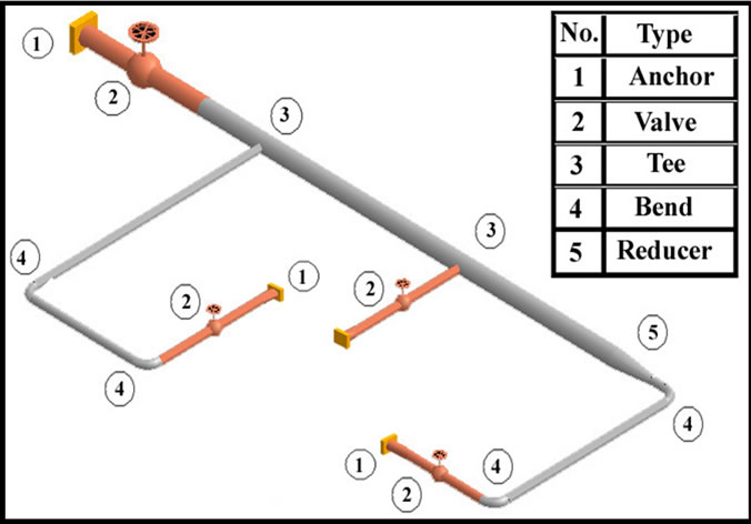
Figure 1. Components of the pipeline model.
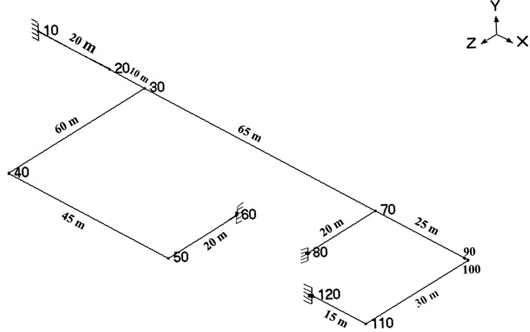
Figure 2. Node numbers and lengths of the pipeline model.
made of the same material of pipeline (SS A53 Grade A). It is also assumed that the three ends of the pipeline are fixed at nodes 60, 80 and 120.
A node refers to a connecting point between elements such as pipes, reducers, valves, and so on. A node has a numeric designation. For bend nodes, the node number is followed by a letter such as A/B. A and B nodes (e.g., 110A, 110B) designate the near and far end of a bend node. Node number refers to the location of the tangent intersection point (TIP); it is not physically located on the bend. Its purpose is only to define the bend. Soil modeling is based on Winkler’s soil model of infinite closely spaced elastic springs. Soil stiffness is calculated for all three directions at each node. Pressure value in the load is suitably modified to consider the effect of static overburden soil pressure [19].
3.2. Components of Pipeline Model
An anchor, is a type of support used to restrain the movement of a node in the three translational and the three rotational directions (or degrees of freedom; each direction is a degree of freedom) [19]. In a piping system, this node may be on an anchor block or a foundation, or a location where the piping system ties into a wall or a large piece of equipment like a pump. The term pipeline bend refers to all elbows and bends. Geometrically, a bend is a curved pipe segment which turns at an angle (typically 90˚) from the direction of the run of the pipe. Reducers change the diameter in a straight section of pipe [20]. Valves are used to control the fluid flow through the pipelines. A valve may be used to block flow, throttle flow, or prevent flow reversal [21].
4. Analytical Steps for Piping Vibration
The key analytical step is to determine, mode by mode, the ratio of maximum dynamic stress to maximum vibration velocity. This ratio will lie in a lower baseline range for uncomplicated systems such as classical uniformbeam configurations. For more complex systems, the Stress/Velocity ratio will increase due to typical complications such as three-dimensional layout, discrete heavy masses, changes of cross-section and susceptible branch connections. System modes with large stress-velocity ratios are the potentially susceptible modes [17]. The Stress/Velocity method implemented in CAEPIPE as the dynamic susceptibility feature automatically and quickly finds these modes and quantifies the susceptibility. Evaluation of the results helps to identify which details of layout and support are responsible for the large stresses [17]. The general susceptibility of a system to large dynamic stresses can be assessed by determining the extent to which the σ/v ratios for any mode exceed the baseline range. Furthermore, by determining which particular modes have the high ratios, and whether these modes are known or likely to be excited, the at-risk vibration frequencies and mode shapes are identified for further assessment and attention. This is the basis of the Stress/ Velocity method of analysis and its implementation as the dynamic susceptibility feature in CAEPIPE.
The dynamic stresses table (like Table 3) provides the distribution of the dynamic stresses around the system, i.e. in effect, the mode shape of dynamic stresses to go along with the conventional mode shape of vibration. This information allows identification of other parts of the system, if any, with dynamic stresses comparable to the identified maximum.
There are two main types of analyses. The first is conceptual, where the structure does not yet exist and the analyst is given reasonable leeway to define geometry, material, loads, and so on. The second analysis is where the structure exists, and it is this particular structure that must be analyzed [22]. Our pipeline model analysis is of the second type.
5. Forced Vibrations of the Mode
In the following cases time history and response spectrum analysis is performed for the pipeline model. Time history force is a function of time at all changes in directions (bends/tees). These separate force-time histories are then applied separately as Time Varying Loads in CAEPIPE at the corresponding nodes in the piping model. Time functions describe the variation of the forcing function with respect to time. A study of an earthquake effects is presented using response spectrum technique.
5.1. The Response Spectrum of an Earthquake Excitation
The earthquake safety of buried pipelines has attracted a great deal of attention in recent years. Important characteristics of buried pipelines are that they generally cover large areas and are subject to a variety of geotectonic hazards. Another characteristic of buried pipelines, which distinguishes them from above-ground structures and facilities, is that the relative movement of the pipes with respect to the surrounding soil is generally small and the inertia forces due to the weight of the pipeline and its contents are relatively unimportant. Buried pipelines can be damaged either by permanent movements of ground (i.e. PGD) or by transient seismic wave propagation.
The concept of response spectrum, in recent years has gained wide acceptance in structural dynamics analysis, particularly in seismic design. Stated briefly, the response spectrum is a plot of the maximum response (maximum displacement, velocity, acceleration or any other quantity of interest), to a specified loading for all possible single degree-of-freedom systems. The abscissa of the spectrum is the natural frequency (or period) of the system, and the ordinate, the maximum response. One of the widely used methodologies for describing the behavior of a structural system subjected to seismic excitation is the response spectrum modal dynamic analysis [23]. Several modal combination rules are proposed in the literature to combine the responses of the individual modes in a response spectrum dynamic analysis [23].
In general, response spectra are prepared by calculating the response to a specified excitation of single degree-of-freedom systems with various amounts of damping [17]. Numerical integration with short time steps is used to calculate the response of the system. The step by step process is continued until the total earthquake record is completed and becomes the response of the system to that excitation. Changing the parameters of the system to change the natural frequency, the process is repeated and a new maximum response is recorded. This process is repeated until all frequencies of interest have been covered and the results can be plotted.
Since the response spectra give only maximum response, only the maximum values for each mode are calculated and then superimposed (modal combination) to give total response. A conservative upper bound for the total response may be obtained by adding the absolute values of the maximum modal components (absolute sum). However this is excessively conservative and a more probable value of the maximum response is the square root of the sum of squares (SRSS) of the modal maxima. In the SRSS method, displacements, element forces, and support loads from the three X, Y and Z accelerations are squared individually and added [17]. The square roots of these respective sums are the displacement, element force and moment, and support load at the given node. To calculate the response of the piping system, for each natural frequency of the piping system, the input spectrum is interpolated. The interpolated spectrum values are then combined for the X, Y and Z directions (direction sum) as SRSS sum to give the maximum response of a single degree-of-freedom system.
5.2. The Time History Excitation
Any phenomenon that gives rise to loads that vary with time can be input into the software CAEPIPE for time history analysis to get the variation of forces or moments with respect to time at different points in the piping system [17]. Time functions describe the variation of the forcing function with respect to time. The actual value of the time function at any time is found by linear interpolation between time points. Time history analysis requires the solution of the equations
 (1)
(1)
where:
[M] = diagonal mass matrix
[C] = damping matrix
[K] = stiffness matrix
{u} = displacement vector
{u} = velocity vector
{u} = acceleration vector
{F(t)} = applied dynamic force vector
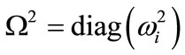
The time history analysis is carried out using mode superposition method. It is assumed that the structural response can be described adequately by the p lowest vibration modes out of the total possible n vibration modes and p < n. Using the transformation u = ΦX, where the columns in  are the p mass normalized eigenvectors, Equation (1) can be written as:
 (2)
(2)
where 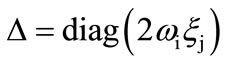
In Equation (2), it is assumed that the damping matrix [C] satisfies the modal orthogonality condition

Equation (2) therefore represents p uncoupled second order differential equations. These are solved using the Wilson  method, which is an unconditionally stable step-by-step integration scheme. The same time step is used in the integration of all equations to simplify the calculations.
6. Excitation Forces
6.1. Response Spectrum of an Earthquake
A direct analytical approach to the problem of the earthquake analysis is to subject the pipeline model to accelerations as recorded in actual earthquakes [24]. The energy content of an earthquake is defined by a response spectrum curve, which plots acceleration (G) vs the frequency in Hz. G is a variable represents the acceleration magnitude correlating to the resultant seismic forces on the equipment [25]. Figure 3 shows the relation between natural frequency (Hz) & Acceleration (G) for the 1940 El Centro earthquake which had a magnitude of 6.4 [26].
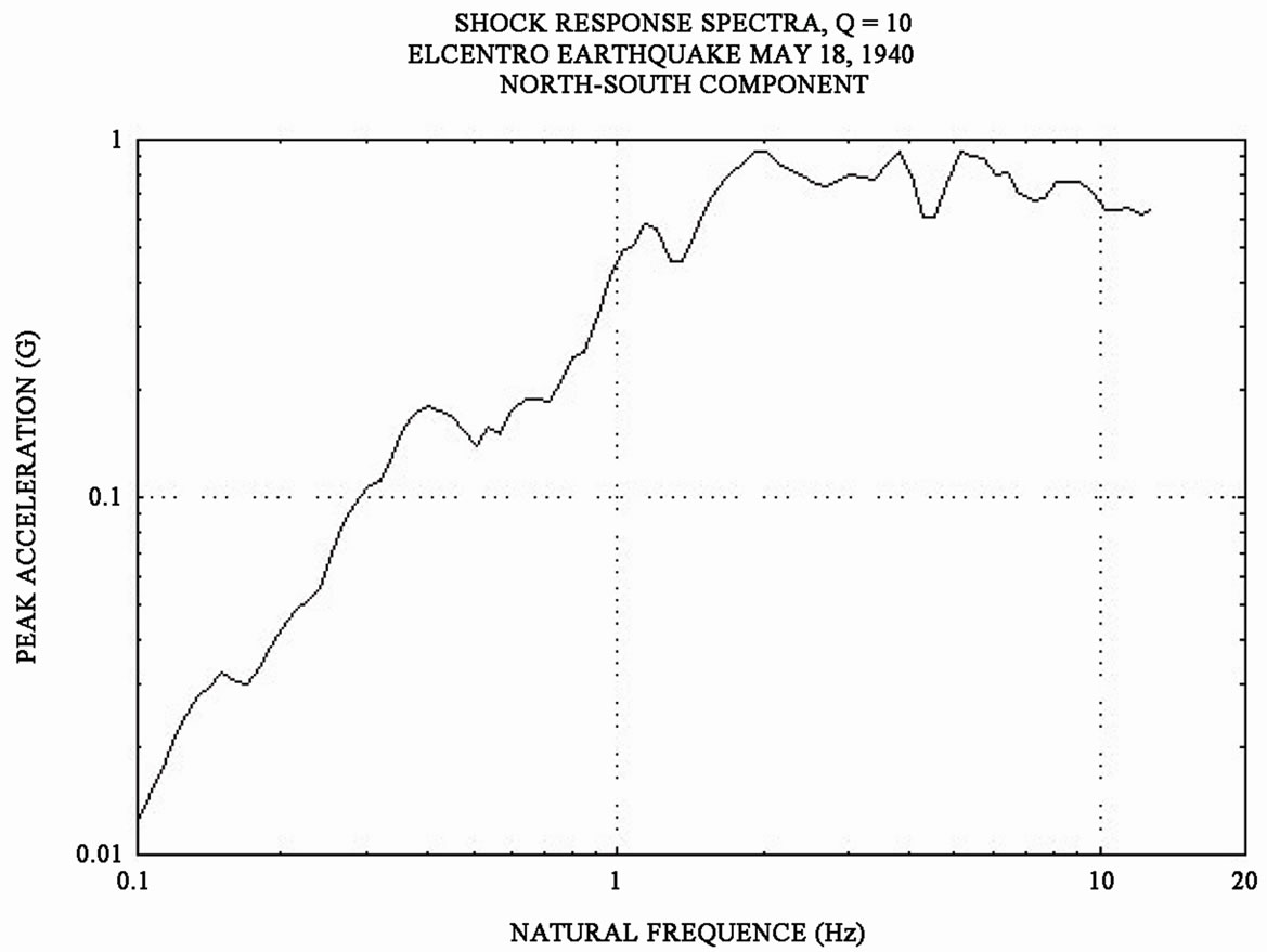
Figure 3. Natural frequency versus acceleration.
Figure 4 shows the input of spectrums and the spectrum load which is applied in the Z-direction. Earthquake load components are applied in both the X and Z directions.
6.2. Time History Analysis of a Truck Crosses the Pipeline
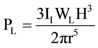
The vertical soil pressure exerted on the pipeline (PL) which caused by two 16,000 lb wheel loads cross simultaneously over the pipe is obtained [27]. The calculated load is for a certain time, for time history analysis. Time will be divided into 10 time steps. Assume the vehicle speed is 40 Km/hr = 11.11 m/s. Equation (3) is called Boussinesq’s equation which can be used to determine the vertical soil pressure from the multiple wheel loads along the pipe [28]
 and
and 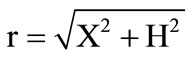 (3)
(3)
whereII: impact factor;
CH: load coefficient;
WL: wheel load;
L: pipe length;
D: pipe outside diameter;
H: vertical depth to point on the pipe crown;
r: distance from the point of load application to the pipe crown.
Figure 5 shows a truck crosses simultaneously over the buried pipeline, and Figure 6 shows different positions for the truck during time intervals.
It can be noticed that load varies with time so we put values into the CAEPIPE software for time history analysis. These loads are input as time functions which are applied to node 90 of pipeline model as time varying loads in the dialogue box in Figure 4. In node 90, the section is reduced and this node is also near the pipeline bend so it can be considered as a weak point in pipeline.
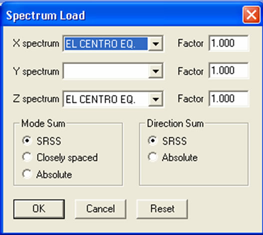
Figure 4. Spectrum loads in X and Z directions of El Centro earthquake.
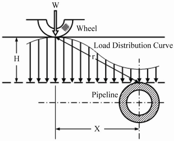
Figure 5. A truck crosses simultaneously over the buried pipeline.
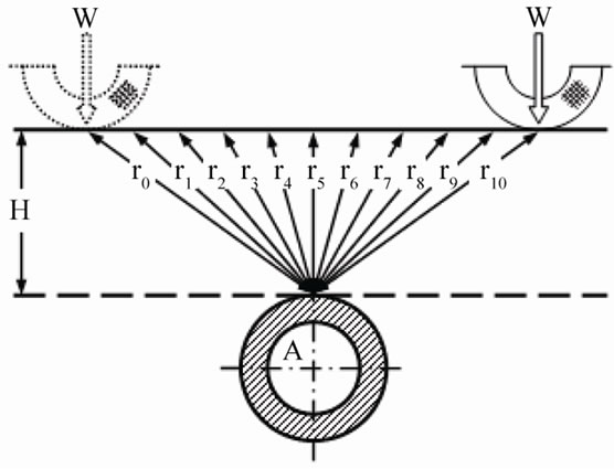
Figure 6. Different positions for the truck during time intervals.
7. Results and Discussion
7.1. Results of Dynamic Susceptibility
Table 1 shows the computed twenty natural frequencies of the constructed mathematical model of the free and supported ends buried gas pipeline, using a finite element program. It’s to notice that the natural frequencies of the supported ends pipeline model are higher than that of the free ends pipeline model, since the later has lower equivalent stiffness than the first one. One can see that the important natural frequencies of the supported ends pipeline system lie between 35 and 71 Hz which can be excited through an excitation of an actual or real object with rotating speeds between 2160 and 4251 rpm.
The following computational work is carried out only for the supported ends model, because it is the most used case, where the output ends are connected to the buildings terminals. The relevant features of this pipeline model can be summarized in Table 2 and the graphic diagrams of some mode shapes in Figures 7-9. In Table 2, mode shapes will be sorted in the order of decreasing susceptibility ratios. The table provides the Stress/Vibration (σ/v) ratios, mode by mode, in rank order of decreasing magnitude. In addition to modal frequencies and σ/v ratios, the table also includes the node locations of
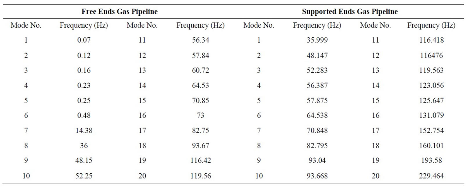
Table 1. The twenty computed natural frequencies for free and supported ends pipeline.
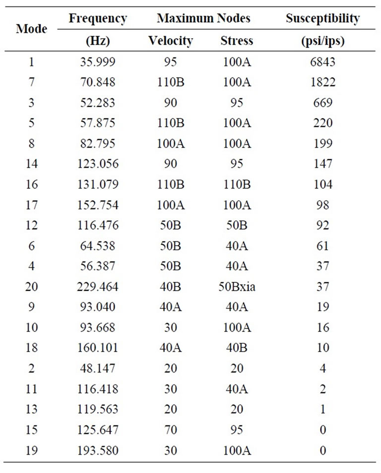
Table 2. Susceptibility ratio and location of max stress and max velocity of every mode shape.
the maximum vibration amplitude and bending stresses.
Figures 7-9 show the graphic display of some vibration mode shapes including the spot markers showing the locations of the maximum vibration velocity (l) and the maximum dynamic bending stress (n) for every mode shape of the pipeline. The following dynamic stresses shown in Tables 3-6 provide the distribution of dynamic stresses of the system for the mode shapes number 1, 7, 3, and 5, i.e. in effect, the mode shapes of
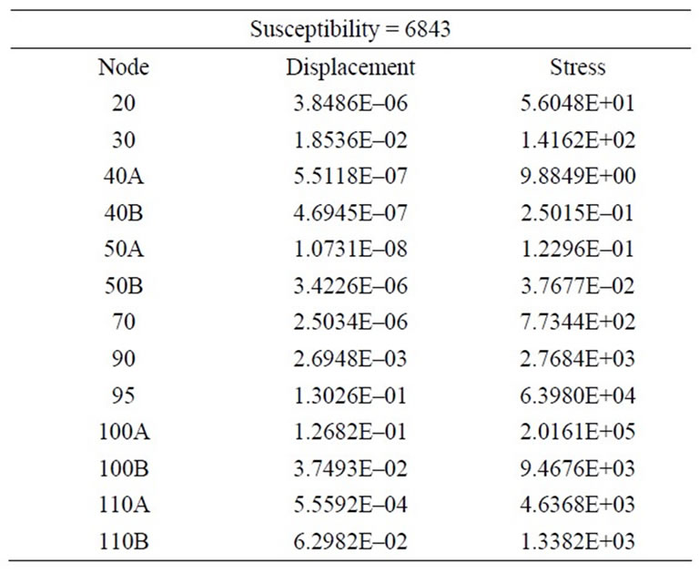
Table 3. Dynamic stresses of mode shape No. 1 (36 Hz).
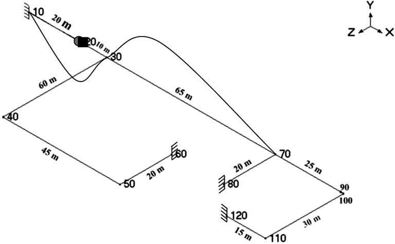
Figure 7. Second mode shape of supported ends pipeline with a natural frequency of 48.147 Hz.
the dynamic stresses to go along with the conventional mode shapes of vibration. From the obtained results, it is shown that some particular modes have high Susceptibil-
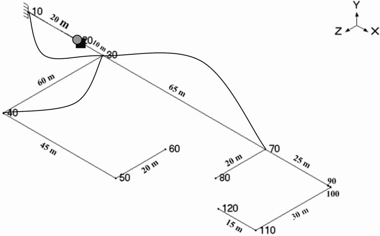
Figure 8. The thirteenth mode shape of supported ends pipeline with a natural frequency of 119.56 Hz.
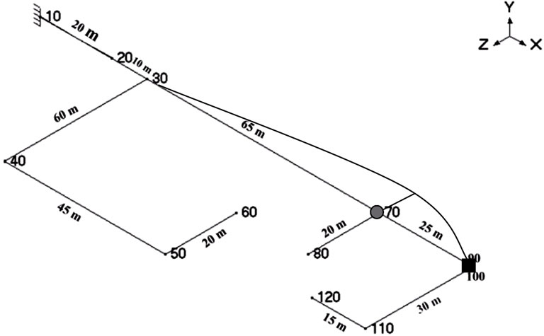
Figure 9. The fifteenth mode shape of supported ends pipeline with a natural frequency of 125.65 Hz.
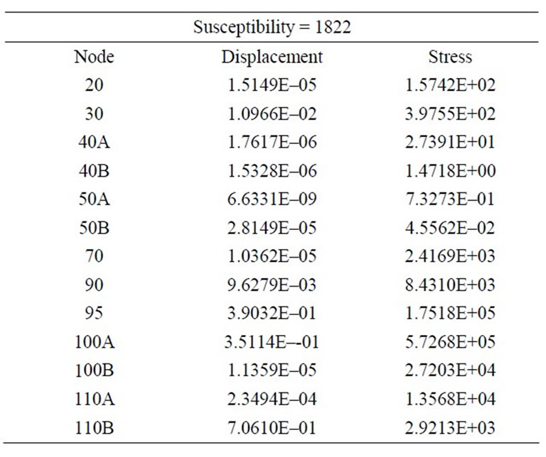
Table 4. Dynamic stresses of mode shape No. 7 (71 Hz).
ity ratios like modes 1, 7, 3 and 5. Causes for increasing ratios can be one or more of the following: large unsupported masses, high-density contents in thin-walled pipe, susceptible branch connections, and changes of pipeline cross sections.
From Table 2 one can see that, while the following
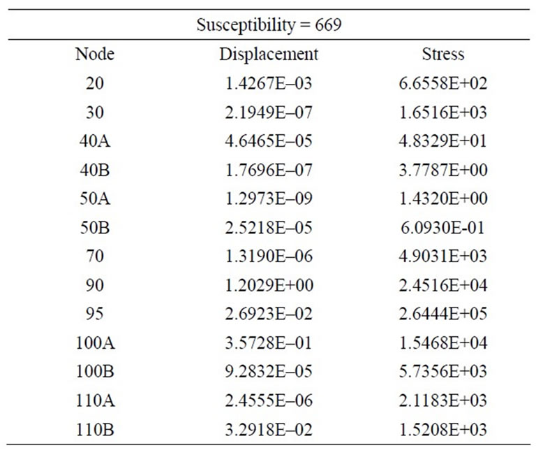
Table 5. Dynamic stresses of mode shape No. 3 (52 Hz).
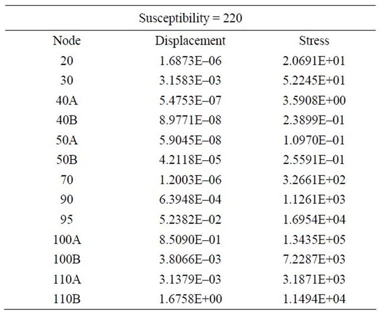
Table 6. Dynamic stresses of mode shape No. 5 (58 Hz).
modes 1, 7, 3, and 5 have the maximum susceptibility ratios (6843 - 669) in the pipeline model, they have the lowest frequencies range (36 - 71 Hz). That is because susceptibility ratio increases with the decreasing of the maximum vibration velocity, and respectively decreasing of the natural frequencies. Modes number 1, 7, 3, and 5 can be described as the at-risk vibration frequencies and mode shapes which need to more attention, by searching for a damping or control methods to limit the dynamic displacements in the piping system to a permissible range.
At the design stage, the dynamic susceptibility feature allows the designer to quickly determine whether the system may be susceptible to very large dynamic stresses. On identifying high susceptibility, the designer can then make changes to improve the design. Locations for measurement of vibration or dynamic strain can be selected based upon knowing the locations of the maximum and the distribution of vibration and dynamic stress. Furthermore, mode-specific acceptance criteria can be readily established to avoid the restrictions of generally over-conservative guideline type criteria, while providing assurance that any highly-susceptible situations are identified and addressed.
7.2. Results of Forced Vibrations of Pipeline Model
Table 7 shows the calculations of the vertical soil pressure on a pipeline model due to a concentrated load at each time interval. Figure 10 is the vertical soil pressure on the pipeline versus time. Figure 11 explains the relation between the distances from the point of load application to the pipe crown and time.
Calculated PL is the load from each wheel; however, the load on the pipe crown is from both wheels, thus (2 PL) is the required value.
7.2.1. Support Loads
Forces and moments on all the supports in the pipeline
Table 7. Calculation of the vertical soil pressure on a pipeline model due to a concentrated load at each time interval.
Figure 10. The relation between the vertical soil pressure on the pipeline (PL) and time.
Figure 11. The relation between the distances from the point of load application to the pipe crown and time.
model are shown in the Table 8. Time history analysis shows that the anchors are subjected to approximately zero forces and low moments about X and Z directions while in response spectrum analysis of the earthquake they are subjected to forces in directions X and Z without moments. In these cases, the force value on any anchor is less than 1 kN and anchors adjacent to loops can be considered strong.
7.2.2. Pipeline Element Forces
The forces and moments on all the pipe elements are computed in global coordinates. Connections to valves are able to resist the pipeline element forces.
7.2.3. Pipeline Element Displacements
Displacements for all load cases are computed in mm in X, Y, Z and in degrees in XX, YY, and ZZ. Dynamic loading cases lead to a little increasing in displacement (less than 1 mm) when comparing with dead loading displacements. Table 9 includes displacements at node 90 for time history analysis using time step 0.1 second and 11 time steps are used to study different displacements within one second. Maximum time history displacement occurs at node 90 as expected, when the truck is located directly over the node 90. The analysis of the earthquake response spectrum displacements shows that there are no additional displacements in support locations and pipeline element movements can be considered in acceptable seismic ranges.
7.2.4. Response Accelerations Act on the Pipeline Due to the Earthquake Excitation
When the acceleration acts on the pipeline, the pipeline experiences this acceleration as a force. The force we are most experienced with is the force of gravity, which caused us to have weight. The units of acceleration are expressed in terms of G (the acceleration due to gravity) and are shown in the Table 10 for different pipeline ele-
Table 8. Support loads.
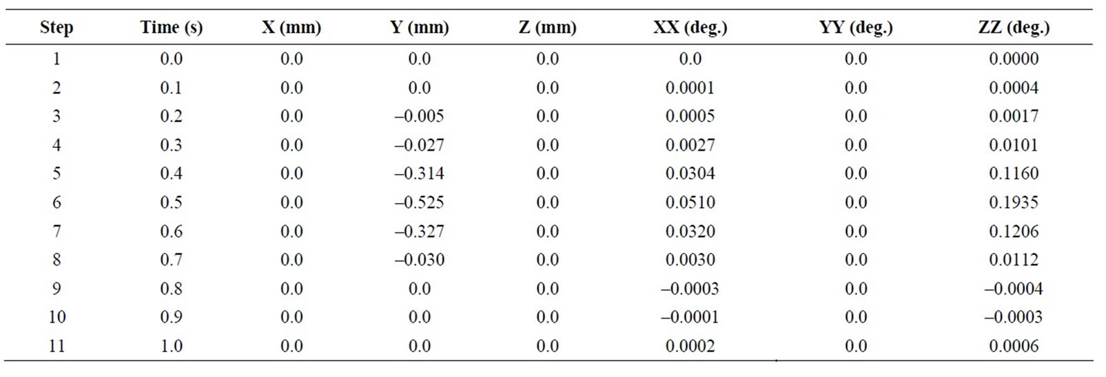
Table 9. Displacements of node 90 for the time history analysis.
ments in X, Y, and Z directions. Response spectrum analysis showed that the pipeline acceleration movements due to EL CENTRO earthquake are in acceptable seismic ranges (Table 10).
8. Conclusions
The behavior of buried gas supply pipelines for free vibration, dynamic susceptibility, and also forced vibration as it is subjected to some external effects like earthquake and truck crosses over the buried pipeline has been investigated. The work summarized has led to a number of conclusions which help in understanding the performance of buried pipelines. Contributions can be summarized in the following main areas:
• The natural frequencies of the supported ends pipeline model are higher than that of the free-ends pipeline model.
• The Stress/Velocity method, implemented in CAEPIPE as the “Dynamic Susceptibility” feature, provides quantified insights into the stress versus vibration characteristics of the system layout.
• In particular, the dynamic susceptibility table identifies specific modes that are susceptible to large dynamic stresses for a given level of vibration. The larger the Stress/Velocity ratio, the stronger the indication that some particular feature of layout, mass distribution, supports, stress raisers etc is causing susceptibility to large dynamic stresses.
• The animated mode-shape display identifies, by the spot-markers, the locations of the respective maxima in dynamic stress and vibration velocity. Review of these animated plots will reveal the offending pattern of motion, and provide immediate insight into what features of the system are responsible for the large dynamic stresses.
• The “dynamic stresses” table provides the distribution of dynamic stresses around the system, i.e. in effect,
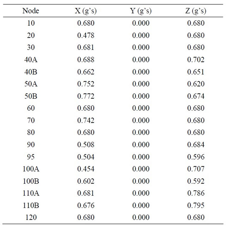
Table 10. Response accelerations act on the pipeline due to the earthquake excitation.
the mode shape of dynamic stresses to go along with the conventional mode shape of vibration. This information allows identification of other parts of the system, if any, with dynamic stresses comparable to the identified maximum.
• The dynamic susceptibility feature of the piping vibration was illustrated here by an application to the pipeline model using the program CAEPIPE. The modal analysis was performed for the frequencies up to 230 Hz, resulting in a reporting-out for 20 modes. The frequency range of (36 - 71 Hz) represents certain modes, which can be considered as important. Graphic displays of the vibration mode shapes including the spot markers showing the locations of the maximum vibration velocity and the maximum dynamic bending stress were illustrated for every mode shape. Previous results enable the designer to quickly determine whether the system may be susceptible to very large dynamic stresses. This could be a broad look at all frequencies, or could be focused on particular frequencies where excitation is likely to occur. Results also can be used for contributing to the planning acceptance testing and the associated measurements where these are undertaken whether by formal requirement or by choice. Locations for measurement of vibration or dynamic strain can be selected based upon knowing the locations of the maxima and the distribution of vibration and dynamic stress.
• Causes for increasing susceptibility ratios can be one or more of the following: large unsupported masses, high-density contents in thin-walled pipe, susceptible branch connections, and changes of pipeline cross sections.
• Time history analysis shows that the anchors are subjected to approximately zero forces and low moments about X and Z directions while in response spectrum analysis of the earthquake they are subjected to forces in directions X and Z without moments.
• Time history analysis showed that the supporting anchors are subjected to moments and a maximum displacement of approximately 0.6 mm occurs when the truck is located directly over the studied point. Response spectrum analysis showed that the pipeline acceleration movements due to El Centro earthquake are in acceptable seismic ranges. For the dynamic loading analysis it is recommended that, the movements should be taken up by bends which have no local stress concentrations and which are so arranged that if yielding occurs there will not be any local failure. For the dynamic loading analysis it is also recommended to avoid subjecting the pipeline components of heavy masses, piping discontinuities, and bends to the expected direct static loads locations as possible.
• Institutions and authorities responsible for the design, construction and operation of buried pipelines located in seismic zones should demand that the seismic effects are correctly taken into consideration in order to assure the good behavior of such pipelines during their working life.
REFERENCES
- Z.-F. Zhang, C.-J. Zhou and L.-Q. Xie, “Pipeline Vibration Reduction of Reciprocating Compressor,” Pipeline Technique and Equipment, Vol. 01, 2006. doi:cnki:ISSN:1004-9614.0.2006-01-006
- T. Chen, Y.-J. Xie, Y.-X. Wang and M. Yu, “Analysis and Transformation of the Vibration of Ketone-BenzolDewaxing Pipelines,” Journal of Liaoning University of Petroleum & Chemical Technology, Vol. 02, 2007. doi:CNKI:ISSN:1672-6952.0.2007-02-013
- C.-B. Fan, L.-B. Zhang, Z.-H. Wang and Y. Tao, “Analysis of Reciprocating Compressor Gas Pipeline Vibration and Control Methods,” Journal of Science Technology and Engineering, Vol. 04, 2007. doi:CNKI:ISSN:1671-1815.0.2007-04-007
- S.-C. Gong, “Analysis on Pipeline Vibration and AntiVibration Measures,” Journal of Coal Technology, Vol. 09, 2004. doi:cnki:ISSN:1008-8725.0.2004-09-069
- C. J. Li and Y. C. Wang, “Analysis of the Vibration in Gas Pipeline System,” Journal of Natural Gas Industry, Vol. 20, No. 2, 2000, pp. 80-83.
- P. Tan, “Analysis on Vibration of Gas Transmission Pipelines,” Journal of Natural Gas Industry, Vol. 01, 2005. doi:cnki:ISSN:1000-0976.0.2005-01-01I
- J. B. Liu, X. H. Zhang, H. Su, C. Sun and Q. C. Zhao, “Finite Element Analysis in Vibration and the Design of the Modified Version for High Pressure Pipe System,” Journal of Daqing Petroleum Institute, Vol. 04, 1996. doi:cnki:ISSN:10001891.0.1996-04-014
- P. Tan, “Analysis of Seismic Response for Gas Pipeline System,” Journal of Natural Gas Industry, Vol. 07, 2005. doi:cnki:ISSN:1000-0976.0.2005-07-035
- R. D. Bao and B. C. Wen, “Study on Seismic Response of Buried Pipeline in Liquefied Soil,” Journal of Earthquake Engineering and Engineering Vibration, Vol. 04, 2008. doi:CNKI:SUN:GCLX.0.2008-04-029
- L. Guha and R. F. Berrones, “Earthquake Effect Analysis of Buried Pipelines,” The 12th International Conference of International Association for Computer Methods and Advances in Geomechanics (IACMAG), 2008, pp. 3957-3967.
- A. El-Kafrawy, “Modal Analysis of Free-Ends Buried Gas Pipelines,” The 9th International Conference, AlAzhar University, Cairo, 2007, pp. 498-513.
- A. El-Kafrawy, “The Dynamic Susceptibility of FixedEnds Buried Gas Pipelines,” The 10th International Mining, Petroleum, and Metallurgical Engineering Conference, Assiut University, Asyut, 2007, pp. 64-83.
- S. G. Kelly and S. K. Kudari, “Mechanical Vibrations,” Tata McGraw-Hill Publishing Ltd., New Delhi, 2007.
- G. Wempner and D. Talaslidis, “Mechanics of Solids and Shells,” CRC Press LLC, Boca Raton, 2003.
- W. C. Young and R. G. Budynas, “Roak’s Formulas for Stress and Strain,” 7th Edition, McGraw-Hill Companies, Inc., New York, 2002.
- K. T. Truong, “Evaluating Dynamic Stresses of a Pipeline,” Mechanical & Piping Division, The Ultragen Group Ltd., Longueuil, 1999.
- “Caepipe Users Manual,” Version 5.1, SST Systems, Appendix E, 2003.
- H. R. Harison and T. Nettleton, “Advanced Engineering Dynamics,” Arnold Hodder Headline Group, London, 1997.
- M. L. Nayyar, “Piping Handbook,” 7th Edition, McGraw-Hill, New York, 2002.
- M. Frankel, “Facility piping systems handbook,” 2nd Edition, McGraw-Hill Companies, Inc., New York, 2002.
- E. W. McAllister, “Pipeline Rules of Thumb Handbook,” 7th Edition, Gulf Professional Publishing, Oxford, 2009.
- J. F. Doyle, “Modern Experimental Stress Analysis,” John Wiley & Sons Inc., New York, 2004. doi:10.1002/0470861584
- P. K. Nukala, “Implementation of Modal Combination Rules for Response Spectrum Analysis,” The University of California, National Technical Information Service, 1999, pp. 1-28. doi:0.2172/10999
- D. Dowrick, “Earthquake Resistant Design and Risk Reduction,” 2nd Edition, John Wiley & Sons Ltd., New York, 2009. doi:10.1002/9780470747018
- G. A. Antaki, “Piping and Pipeline Engineering,” 2005.
- W. F. Chen and C. Scawthorn, “Earthquake Engineering Handbook,” CRC Press LLC, Boca Raton, 2003.
- V. R. Nieves, “Static and Dynamic Analysis of a Piping System,” M.Sc. Thesis, University of Puerto Rico, Mayagues Campus, 2004.
- Chevron Philips Company LP, “Buried Pipe Design,” Appendix D: Book 2, Chapter 7, 2003, pp. 1-36.