Intelligent Control and Automation
Vol. 3 No. 2 (2012) , Article ID: 19239 , 13 pages DOI:10.4236/ica.2012.32017
Regional Controllability of Semi-Linear Distributed Parabolic Systems: Theory and Simulation
1TSI Group, Department of Mathematics and Computer Sciences, Faculty of Sciences, Moulay Ismail University, Meknes, Morocco
2Department of Mathematics, College of Sciences, Al Jouf University, Sakakah, KSA
Email: {as2.kamal, boutouloutali}@yahoo.fr, beinane06@gmail.com
Received March 20, 2012; revised May 2, 2012; accepted May 10, 2012
Keywords: Semi-Linear Parabolic Systems; Regional; Internal/Boundary Controllability; Fixed-Point Theorems; Distributed System; HUM Approach
ABSTRACT
The aim of this brief paper is to give several results concerning the regional controllability of distributed systems governed by semi-linear parabolic equations. We concentrate on the determination of a control achieving internal and boundary regional controllability. The approach is based on an extension of the Hilbert Uniqueness Method (HUM) and Schauder’s fixed point theorem. We give a numerical example developed in internal and boundary sub region. These numerical illustrations show the efficiency of the approach and lead to conjectures.
1. Introduction
Many scientific and engineering problems can be modeled by partial differential equations, integral equations, or coupled ordinary and partial differential equations that can be described as differential equations in infinite-dimensional spaces using semi groups. Nonlinear integrodifferential equations, with and without delays, serve as an abstract formulation for many partial integrodifferential equations which arise in problems connected with heat flow in materials with memory, viscoelasticity, and other physical phenomena. In particular, Sobolev-type equations occur in thermodynamics in the flow of fluid through fissured rocks, in the shear of second-order fluids, and in soil mechanics. So, the study of controllability results for such systems in infinite-dimensional spaces is important.
For the motivation of abstract systems and the controllability of linear systems, one can refer to the books by Curtain and Pritchard [1], and by Curtain and Zwart [2]. For an earlier survey on the controllability of nonlinear systems using fixed-point theorems, including nonlinear delays systems, see [3]. The approximate controllability of nonlinear systems when the semigroup generated by A is compact has been studied also by many authors. The results of Zhou [4] and Naito [5] give sufficient conditions on B with infinite-dimensional range or necessary and sufficient conditions based on more strict assumptions on B. Li and Yong [6] studied the same problem assuming the approximate controllability of the associated linear system under arbitrary perturbation in  Bian [7] investigated the approximate controllability for a class of semi-linear systems, [8] used the Banach fixed-point theorem to obtain a local exact controllability in the case of nonlinearities with small Lipschitz constants. Zhang [9] studied the local exact controllability of semi-linear evolutions systems. Naito [5] and Seidmann [10] used the Schauder fixed-point theorem to prove the invariance of the reachable set under nonlinear perturbations. Klamka [11-13] studied sufficient conditions for constrained exact controllability in a prescribed time interval for semi-linear dynamical systems in which the nonlinear term is continuously Frechet differentiable are formulated and proved assuming that the controls take values in a convex and closed cone with vertex at zero. The method used covers a wide class of semi-linear abstract dynamical systems and is specially useful for semi-linear ones with delays. Balachandran and Sakthivel [14] studied the controllability of semilinear integrodifferential systems in Banach spaces by using the Schaefer fixed-point theorem. Fabre et al. [15] prove approximate controllability in
  for 1 ≤ p <
  by means of a control which can be internal or on the boundary and when the nonlinearity is globally Lipschitz. Other related abstract results were given by Zuazua [16], Lasiecka et al. [17] and Kassara et al. [18].
The study of various analytic concepts related to controllability and stability of such systems is, in general, delicate and considering only linear model can not be sufficient in particular when some properties of system needs to be satisfied only in some part of the system evolution domain. From practical point of view, it is very natural to consider the analysis of such systems only in some subregion of its evolution system domain. This is the aim of regional analysis.
The regional analysis of distributed parameter system has recieved an intensive study in the last three decades.
The term “regional analysis” has been used to refer to control problems in which the target of our interest is not fully specified as a state, but refers only to a smaller region  of the system domain. This concept has been widely developed and interesting results have been obtained, in particular, the possibility to reach a state only on an internal subregion
  of
of  (El Jai et al. [19]) or on a part of the boundary
  of (Zerrik et al. [20]). The principal reason for introducing this concept is that, first it makes sense for the usual controllability concept closer to real world problem and, second, it can be applied to systems which are not controllable on the whole domain. Here we are interested on regional controllability of semi-linear parabolic systems. More precisely the question concerns the possibility of regional controllability for semi-linear system in the case where the desired state is given only on an internal subregion
  of
of  or on a part of the boundary
  of
of .
.
The interest of this work focused on the development of an approach that leads to numerical implementation for the computation of the control which steers the system from an initial state to a given regional internal and boundary state. A typical motivating example is the case of a biological reactor, where the problem is to regulate the concentration of a susbstratum at the bottom of the reactor [21].
In Section 2, first we present some preliminary material and state internal regional controllability problem of semi-linear systems. Next, we concentrate on the determination of a control achieving regional internal controllability, and we develop a numerical approach that leads to a useful algorithm and successfully tested through a diffusion process. Section 3 is focused on the regional boundary target control problem, and an approach is developed that leads to a numerical algorithm for the computation of a control which achieves regional boundary controllability. Numerical illustrations show the efficiency of the approach and lead to conjectures.
2. Regional Internal Controllability
2.1. Statement of the Problem
Let  be a regular bounded open set of IRn,
  with boundary
 . For a given time T > 0, let
 , and
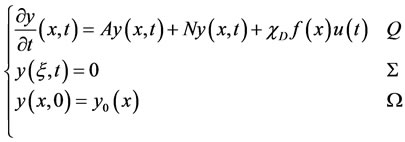
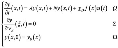
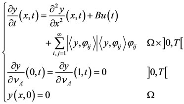
, and  We consider a semi-linear parabolic system excited by controls which can be applied via various types of actuators given by the following equation
 (2.1)
(2.1)
where A is a second-order linear differential operator, which generates a strongly continuous semi-group  on Hilbert space
  and N a locally lipschitz continuous nonlinear operator.
 ,
,  and
and  where
where
where p represents the number of actuators. We denote by U the completion of the space  endowed with the standard norm of
 . Denote by
  the solution of (2.1) when it is excited by a control u, suppose that
 . Let us recall that an actuator is conventionally defined by a couple
  where
where  is the geometric support of the actuator and f is the spatial distribution of the action on the support D, see [22]. In this case,
  In the case of pointwise actuator (internal or boundary),
  and
and , where
  is the Dirac mass concentrated at
  in this case, the actuator is denoted by
  and
and .
.
Let  be the solution of (2.1) excited a control u and assume that
  see [23].
For , open, nonempty and of positive Lebesgue measure, we consider the operator restriction
and  denotes the adjoint operator.
Definition 1
• System (2.1) is said to be  -exactly regionally controllable if for all
  there exists a control
  such that
• System (2.1) is said to be  -approximately regionally controllable if for all
  and for all
 , there exists a control
  such that
The notion of regional controllability considered as a particular case of output controllability was introduced and developed for linear system in (El Jai et al. [19], Zerrik et al. [20]).
It is clear that:
• If system (2.1) is regionally controllable on  then it is regionally controllable on any
• In the linear case, one can find states which are approximately regionally controllable on  but not controllable on the whole domain
 , see [19,22].
To study the controllability of the system (2.1), we consider its corresponding linear system 
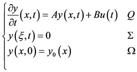 (2.2)
(2.2)
The problem of regional controllability on  for (2.1) can be stated as follows:
Problem
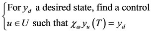 (2.3)
(2.3)
More precisely, it is asked to find a control which steers system (2.1), at time T, to a desired state defined in subregion .
.
2.2. Hilbert Uniqueness Approach
The aim of this section is to give an extension of regional controllability and Hilbert uniqueness method introduced in the linear case by (El Jai et al. [19]) and [24] which allows the characterization of a control  solution of (2.3). The system (2.2) is approximately controllable in
  and system (2.1) is excited by a zone actuator
 . System (2.1) may be rewritten in the form
 (2.4)
(2.4)
and the operator  verify
 (2.5)
(2.5)
Let 
 (2.6)
(2.6)
Which has a unique solution  see [25].
For a given , we consider the system (2.6) and define the mapping
 (2.7)
(2.7)
Which is a norm on G; since the system (2.2) is approximately controllable in .
.
Consider the system
 (2.8)
(2.8)
and the associated linear system
 (2.9)
(2.9)
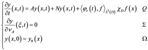
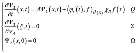
The system (2.8) may be decomposed in the following three systems
 (2.10)
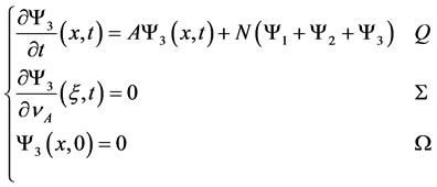
and
 (2.11)
where  is the solution of (2.6) and
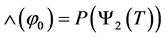
 (2.12)
We denote the completion of the set G with respect to the norm (2.7) again by G.
Let  be defined by
  where
where .
.
Now, with the nonlinear operator

The problem of regional controllability (2.3) turns up to solve the equation  which is equivalent to
where  is the operator defined by the formula
 . Then we have
 (2.13)
The linear system (2.9) is approximately regionally controllable in , then
  is one to one see [19].
Apply  the equation (2.13), we have
Now, we define the nonlinear operator  by
by
 (2.14)
Then the problem (2.3) of system (2.7) turns up to search a fixed point of , then we have
Proposition 1
Assume that (2.5) holds. If the linear system (2.9) is approximately regionally controllable in , then the control
  steers the system (2.8) to
  in
in  at
at  where
where  is the solution of the system (2.6) and
  is a fixed point of the operator
  given by (2.14).
Sketch of the proof: The proof may be easily achieved with the following two steps:
Step 1: We prove that K is a compact operator and then deduce that  is also compact.
Step 2: Applying the Schauder fixed-point theorem, we see that the operator  has a fixed point. For more details we refer the reader to [26].
Remark 1
The above approach is a generalization of the Hilbert uniqueness method given in the linear case  and the operator
  coincides with the isomorphism
 .
.
Algorithm 1
Summing up, in the zone case, the regional controllability is obtained via the following simplified algorithm
• Step 1: we take the following initial conditions ,
,  , f, D and
 .
.
• Step 2: Using the pseudo-code.
■ Resolution of (2.6) and obtaining 
■ Resolution of (2.10) and obtaining 
■ Resolution of (2.11) and obtaining 
■ Resolution of (2.12) and obtaining 
■ Calculation of  and obtaining
 .
.
■ Resolution of  and obtaining
 .
.
■ Until 
• Step 3: The control .
.
2.3. Simulations
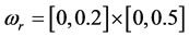
The goal of this section is to test the efficiency of the previous algorithm. The obtained results are related to the considered subregion, the desired state and the actuator structure. Let  and consider the one-dimensional diffusion system described by
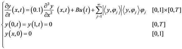 (2.15)
2.3.1. Zone Actuator
In this case  where
where  The subregion under consideration is
 .
.
Let 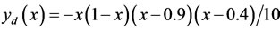 be the desired regional state in
 . Using the previous algorithm1, the simulation gives the Figure 1.
The regional desired state  is reached with error
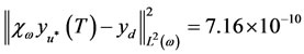
and transfer cost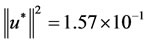 .
.
2.3.2. Pointwise Actuator
In this case  where
where 
We consider the subregion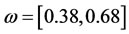 .
.
Let 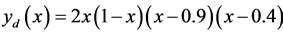 be the desired regional state on
 . The simulation gives the Figure 2.
The regional desired state  is reached with error
and transfer cost .
.
2.3.3. Relation between the Subregion and Location of the Pointwise Actuator
The following simulation results show the evolution of the desired state error with respect to the actuator location. Figure 3 shows that:
• For a given subregion  and a desired state, there is an optimal actuator location (optimal in the sense that it leads to a solution which is very close to the desired state).
• When the actuator is located sufficiently far from the subregion , the estimated state error is constant for any location.
• The worst locations correspond to non strategic actuators in , as developed in the linear case see [19].
Figure 4 shows that, for a given subregion and a desired state, there is an optimal actuator location in the sense that it leads to a smaller transfer cost.
The results are similar for other types of actuators.
3. Regional Boundary Controllability
The aim of this section is to give an extension of the concepts of regional internal controllability [26] to the case where is a part of the boundary of the domain. The developed  method is original and leads to a numerical algorithm illustrated by simulations.
3.1. Considered System and Problem Statement
Let  be a bounded open domain in IRn (n = 1, 2, 3) with a regular boundary
 . For
. For , we write

Figure 1. Desired state (continuous line) and final state (dashed line) on the region ω.
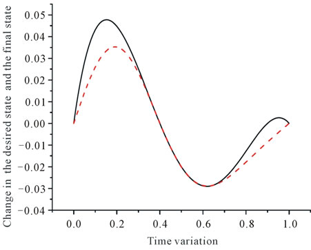
Figure 2. Desired state (continuous line) and final state (dashed line) on the region ω.
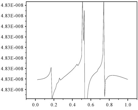
Figure 3. The evolution of the estimated state error with respect to the actuator locations.

Figure 4. The evolution of the transfer cost with respect to the actuator locations.
 ,
, 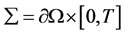 and consider the following semi-linear parabolic system
 (3.1)
(3.1)
where
• A is a second-order linear differential operator, which generates a strongly continuous semi-group  on Hilbert space
 .
.
• N a locally lipschitz continuous nonlinear operator.
• 
•  where
where  with
with  be the solution of (3.1) excited by a control u.
We denote by U the completion of the space  endowed with the standard norm of
 .
.
Assume that  The controls may be applied via various types of actuators see [22].
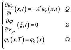
The associated linear system is
 (3.2)
(3.2)
For Γ being a regular subset of  which has positive Lebesgue measure, consider the restriction operator

where  denotes its adjoint operator.
Let us  whilst
  is considered for the adjoint operator.
We introduce the definition.
Definition 2
The system (3.1) is said to be  -exactly (resp.
  - approximately) regionally controllable if for all
 (resp. for all
 ) there exists a control
 such that
  (resp.
  ).
).
This definition generalizes the standard ones of exact and approximate controllability on the whole domain .
.
Remark 2
1) The notion of regional controllability considered as a particular case of output controllability was introduced and developed for linear system in [20].
2) A system which is  -exactly (resp.
  -approximately) regionally controllable is
  -exactly (resp.
  - approximately) regionally controllable for all
 .
.
3) The above definitions do not allow for pointwise or boundary controls since, for such.
4) systems  and the solution
  However, the extension can be carried out in a similar manner if one takes regular controls such that
  [27].
[27].
In the sequel, we explore the possibility of finding a control which ensues the transfer of system (3.1) to desired  on the boundary subregion
  consider the problem
 (3.3)
(3.3)
3.2. Theoretical Approach
Firstly, the following result provides a link between regional internal controllability see [26] and regional boundary controllability for semi-linear systems.
Consider the linear and continuous extension operator
 such that
  for all
  For
For , we denote by
  the extension of
  to
to  and we define

Let integer small, we set
  and
and  , where
  is the open ball of radius r and center z, see [28]. Then, we have the following result.
Proposition 2
If the system (3.1) is  -exactly (resp.
  -approximately) regionally controllable, then it is
  -exactly (resp.
  -approximately) regionally controllable.
Proof
Let  then by trace theorem, there exists
  with a bounded support such that

Since the system (3.1) is  -exactly controllable, then there exists a control
  such that
Thus  and then
  Consequently, the system (3.1) is
  -exactly controllable.
Now, if the system (3.1) is  -approximately controllable, for all
 , there exists
  such that

and by continuity of the trace mapping , we have
therefore
Consequently, the system (3.1) is  -approximately controllable.
Secondly, we develop an approach devoted to characterize a control  solution of problem (3.3), when the system (3.1) is
  -approximately controllable. The approach we shall use is based on an extension of regional controllability techniques for linear systems developed in (El Jai et al. [19]) and Hilbert uniqueness method see [24].
The system (3.2) is excited by a control applied by means of a zone actuator  where
where  is the actuator support and
  defines the spatial distribution of the control on D, then the system (3.2) may be written in the form
 (3.4)
(3.4)
The operator  verify
 (3.5)
(3.5)
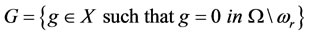
Let G be the set
For , we denote by
  the extension of
  to
to 
Consider the system
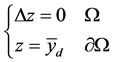 (3.6)
(3.6)
where  is the Laplace operator. The system (3.6) has a unique solution z in
 . Let
. Let  the restriction of z in
The problem of reaching  on
on  may then be solved by reaching
  on
on  Then the problem (3.3) is formulated as follows:
 (3.7)
(3.7)
For , the system
 (3.8)
(3.8)
has a unique solution  [28].
[28].
In G, we define the mapping
 (3.9)
(3.9)
which is a norm on G; since the system is  -approximately controllable see [19].
Consider the system
 (3.10)
and its associated linear system is
 (3.11)
The system (3.10) may be decomposed into the following three systems
 (3.12)
and
 (3.13)
where  is the solution of (3.8) and
 (3.14)
We denote the completion of the set G with respect to the norm (3.9) again by G.
Consider the operator  defined by
 where
where  is the dual of
  and
and 
Let us now define the nonlinear operator

The problem of regional controllability (3.3) turns up to solve the equation
which is equivalent to
where  is the operator defined by
 , which gives
 (3.15)
Since the linear system (3.11) is  -approximately regionally controllable, then
  is one to one see (El Jai et al. [19]).
Apply  the equation (3.15), we have
Then a solution of problem (3.3) of system (3.10) turns up to search a fixed point of nonlinear operator  define by
 (3.16)
Then we have:
Proposition 3
If the linear system (3.11) is  -approximately regionally controllable, then the control
 drives the system (3.10) to
in  at
at , where
  is the solution of the system (3.9) and
  is a fixed point of the operator
  given by (3.16).
Proof
Step 1: We prove that  is a compact operator.
Let the ball  in X, we have
 and we set

Where  is solution of the system (3.14).
We have
 (3.17)
 see [23] and there exists
  such that
Since  is a strongly continuous semi-group on
 , then there exists
  such that
and from (3.17), we have

Since  is solution of the system (3.12), then
  and we have
 (3.18)
Since  is solution of the system (3.13), then we have
and

then
 (3.19)
thus

By Gronwall’s lemma, we obtain
 (3.20)
then
Hence,  is uniformly bounded.
Let show that  is relatively compact, indeed: for
  and
and , we have

where
and
For all , there exists
  such that

which gives
from (3.18), (3.19) and (3.20), we have

and


Thus

where
and
For  and
and , we obtain
  Then,
Then,  is relatively compact.
Finally, by the Arzelà-Ascoli theorem see [29,30],  is a compact operator, then
  is also compact.
Step 2: From (3.16) and (3.20), we have
where

and

The constant  verify

It is being used the fact that  is small.
Let  such that
 , then we have

 such that
 .
.
Hence, by applying Schauder’s fixed point theorem see [30], the operator  at least one fixed point, and the proof is completed.
Algorithm 2
With the same hypothesis as in the last section, we have the following algorithm
• Step 1: we choose the initial conditions, subregion ,
,  ,
,  , and the function
 , D and
 .
.
• Step 2: using the pseudo-code.
■ Resolution of (3.8) and obtaining 
■ Resolution of (3.12), (3.13) and (3.14)
■ Calculation of  and obtaining
 .
.
■ Resolution of  and obtaining
 .
.
■ Until 
• Step 3: The control .
.
3.3. Numerical Example
In this subsection, we present a numerical example which illustrate the previous algorithm. It shows that there exists a link between the subregion area and the reached state error, the results are related to the choice of the subregion and the desired state to be reached.
Consider the two-dimensional diffusion system
 (3.21)
3.3.1. Zone Actuator
We consider
• The actuator is located in
 .
.
•  ,
, : Intern subregion target.
•  : Boundary subregion target.
•  : The desired state to be reached in
•  : The extension of desired state
  on
on 
• Using the previous algorithm 2 in the case zone actuator we have Figures 5-8.
Using the previous algorithm, the regional desired state  is obtained with error
and cost 
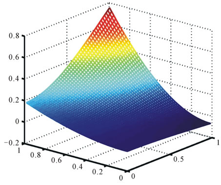
Figure 5. Desired state on the region ωr.
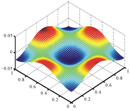
Figure 6. Final state on the region ωr.
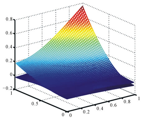
Figure 7. Desired and final state on the region ωr.
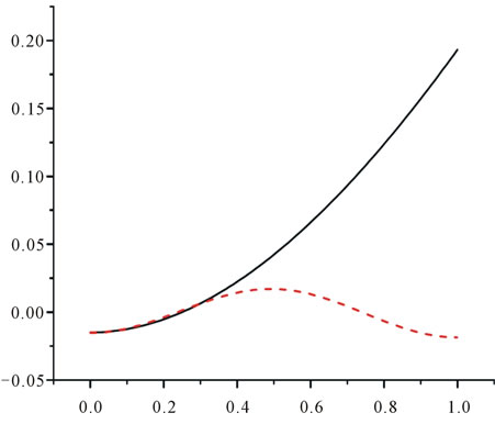
Figure 8. Trace of desired and final state on the region Γ.
3.3.2. Relation between the Subregion Area and Reached State Error
The reached state error depends on the area of the subregion where the desired state has to be given. This error grows with the subregion area. It means that the larger the region is, the greater the error is (see Table 1).
The results are similar for other types of actuator.
3.3.3. Pointwise Actuator
In this case, we have
• The actuator is located in  with b1 = 0.162,
•  ,
,  Intern subregion target.
• 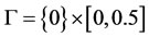 : Boundary subregion target.
•  : The desired state to be reached in
•  : The extension of desired state
  on
on 
• Using the previous algorithm 2 in the case point wise actuator we have Figures 9-12.
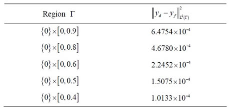
Table 1. The relation between the subregion area and reached state error.

Figure 9. Desired state on the region ωr.
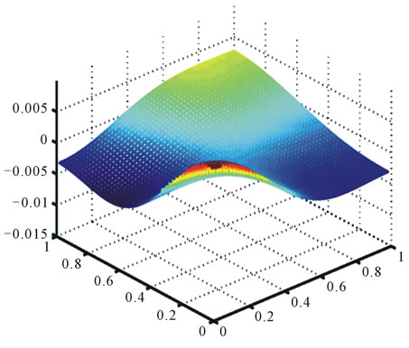
Figure 10. Final state on the region ωr.

Figure 11. Desired and final state on the region ωr.
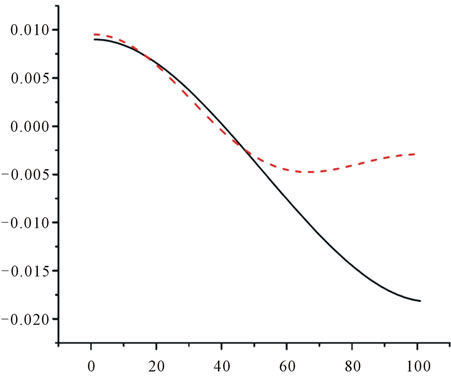
Figure 12. Trace of desired and final state on the region Γ.
4. Conclusions
The work is provide an interesting tool to achieve regional internal and boundary target for a semi-linear parabolic system excited by actuator. The problems of regional controllability are solved using linear regional controllability techniques and by applying HUM method and fixed point theorems. The obtained result leads to an algorithm which was implemented numerically. Examples of various situations and simulations are given.
Various open questions are still under consideration. For example, this is the case of the problem where we test this algorithm for real applications. This case is presently being studied and the results will appear in a separate paper.
The problem of regional controllability problem for semi-linear parabolic systems with time delays is of great interest and the work is under consideration and will be the subject of the feature paper.
REFERENCES
- R. F. Curtain and A. J. Pritchard, “Infinite-Dimensional Linear Systems Theory, Lecture Notes in control and information sciences,” Springer Verlag, Berlin, 1978.
- R. F. Curtain and H. Zwart, “An introduction to Infinite Dimensional Linear Systems Theory,” Springer Verlag, Berlin, 1995.
- K. Balachandran and J. P. Dauer, “Controllability of Nonlinear Systems via Fixed-Point Theorems,” Journal of Optimization Theory and Applications, Vol. 53, No. 3, 1987, pp. 345-352. doi:10.1007/BF00938943
- H. Zhou, “Approximate controllability for a class of semilinear Abstract Equations,” SIAM Journal on Control and Optimization, vol. 21, No. 4, 1983, pp. 551-555. doi:10.1137/0321033
- K. Naito, “Approximate controllability for trajectories of Semilinear Control Systems,” Journal of Optimization Theory and Applications, vol. 60, No. 1, 1989, pp. 57-65. doi:10.1007/BF00938799
- X. Li and J. Yong, “Optimal Control Theory for InfiniteDimension a systems,” Birkhauser, Basel, 1994.
- W. M. Bian, “Constrained controllability of some nonlinear systems,” Applicable Analysis, vol. 72, No. 1-2, 1999, pp. 57-73. doi:10.1080/00036819908840730
- N. Carmichael and M. D. Quinn, “Fixed-Point Methods in Nonlinear Control, Lecture notes in Control and Information Sciences,” Springer Verlag, Berlin, 1984.
- X. Zhang, “Exact controllability of Semilinear Evolution Systems and Its Application,” Journal of Optimization Theory and Applications, vol. 107, No. 2, 2000, pp. 415- 432. doi:10.1023/A:1026460831701
- T. I. Seidmann, “Invariance of the Reachable Set under Nonlinear Perturbations,” SIAM Journal on Control and Optimization, vol. 25, No. 5, 1985, pp. 1173-1191. doi:10.1137/0325064
- J. Klamka, “Constrained Approximate Controllability,” IEEE Transactions on Automatic Control, vol. 45, No. 9, 2000, pp. 1745-1749. doi:10.1109/9.880640
- J. Klamka, “Schauder’s Fixed-Point Theorem in Nonlinear Controllability Problems,” Control and Cybernetics, vol. 29, No. 1, 2000, pp. 153-165.
- J. Klamka, “Constrained controllability of Semilinear Systems,” Nonlinear Analysis, vol. 47, No. 6, 2001, pp. 2939-2949. doi:10.1016/S0362-546X(01)00415-1
- K. Balachandran and R. Sakthivel, “Controllability of Integrodifferential Systems in Banach Spaces,” Applied mathematics and optimization, vol. 118, No. 1, 2001, pp. 63-71. doi:10.1016/S0096-3003(00)00040-0
- C. Fabre, J. P. Puel and E. Zuazua, “Approximate controllability of the Semilinear Heat Equation”, Proceedings of the Royal Society of Edinburgh: Section A Mathematics, Vol. 125, No. 1, 1995, pp. 31-64. doi:10.1017/S0308210500030742
- E. Zuazua, “Contrôlabilité exacte d'un modèle de plaques vibrantes en un temps Arbitrairement Petit,” Comptes rendus de l’Académie des sciences, vol. 304, no. 7, 1987, pp. 173-176.
- I. Lasiecka and R. Triggiani, “Exact controllability of Semilinear Abstract Systems with applications to waves and Plates Boundary Control Problems,” Applied mathematics and optimization, vol. 23, No. 1, 1991, pp. 109- 154. doi:10.1007/BF01442394
- K. Kassara and A. El Jai, “Algorithme pour la commande d’une classe de systèmes à paramètres répartis non linéaires,” Applied mathematics and optimization, vol. 1, 1993, pp. 3-24.
- A. El Jai, A. J. Pritchard and E. Zerrik, “Regional controllability of Distributed Systems,” International Journal of Control, Vol. 62, No. 6, 1995, pp. 1351-1365. doi:10.1080/00207179508921603
- E. Zerrik, A. Boutoulout and A. El Jai, “Actuators and Regional Boundary Controllability of Parabolic Systems,” International Journal of Systems Science, vol. 31, No. 1, 2000, pp. 73-82. doi:10.1080/002077200291479
- J. Jacob, “Modélisation et simulation dynamique de procédés des eaux de type biofiltre. Traitement d'équations différentielles partielles etalgébriques,” Thése de Doctorat I. N. P., Toulouse, 1994.
- A. El Jai and A. J. Pritchard, “Capteurs et actionneurs dans l’analyse des systèmes distribués,” Masson, Paris, 1986.
- A. Pazy, “Semigroups of Linear Operators and applications to Partial Differential Equations,” Springer-Verlag, Berlin, 1983.
- J. L. Lions and E. Magenes, “Problèmes aux limites non homogènes et applications,” Dunod, Paris, 1968.
- E. Zerrik and A. Kamal, “Output controllability for semi-linear Distributed Parabolic Systems,” Journal of Dynamical and Control Systems, vol. 13, No. 2, 2007, pp. 289-306. doi:10.1007/s10883-007-9014-8
- A. El Jai and A. J. Pritchard, “Sensors and actuators in Distributed Systems Analysis,” Ellis horwood, Chichester, 1988.
- A. El Jai, “Eléments de contrôlabilité,” Presses Universitaires de Perpignan, Perpignan, 2006.
- J. L. Lions, “Contrôlabilité exacte, Perturbations et stabilisation des systèmes distribués,” Masson, Paris, 1988.
- H. Brezis, “Analyse fonctionnelle: théorie et application,” Masson, Paris, 1983.
- E. Zeidler, “Applied Functional Analysis: Applications to mathematical physics,” Springer-Verlag, Berlin, 1995.