Materials Sciences and Applications
Vol.10 No.08(2019), Article ID:94458,16 pages
10.4236/msa.2019.108041
Applicability of Strain Controlled Cyclic Tests for Short Fibre Reinforced Polymers
Andreas Primetzhofer1*, Garbriel Stadler2, Gerald Pinter1,3, Florian Grün2
1Polymer Competence Center Leoben GmbH (PCCL), Leoben, Austria
2Montanuniversität Leoben, Chair of Mechanical Engineering, Leoben, Austria
3Montanuniversität Leoben, Chair of Materials Science and Testing of Polymers, Leoben, Austria

Copyright © 2019 by author(s) and Scientific Research Publishing Inc.
This work is licensed under the Creative Commons Attribution International License (CC BY 4.0).
http://creativecommons.org/licenses/by/4.0/


Received: June 24, 2019; Accepted: August 18, 2019; Published: August 21, 2019
ABSTRACT
To develop parts, made of short glas fibre reinforced (sgfr) polymers for industrial purposes, a comprehensive material knowledge is necessary. Especially the material behaviour under cyclic loads has a great influence on the life time of parts. Parts are often used under complex load cases (stress state, temperature, ...), therefore it is indispensable to understand the effect of the main influence factors. High loads within load histories as well as stress concentrations can lead to plastic deformations. To cover this in an early stage of the development process, a closed simulation chain should be established. Therefore, the applicability of common material models (e.g. fatigue criteria according to Ramberg-Osgood) has to be studied first, the models have to be adapted or even new models have to be found for sgfr materials. This work focuses on the applicability of strain controlled cyclic tests for glass fibre reinforced polymers. Hereby the cyclic stress rearrangement in the low cycle regime of the S/N-curve can be described. Therefore, tests were performed on a 50 wt% sgfr partial aromatic polyamide. For the fatigue tests un-notched, injection moulded specimen were used. The tests show a principal applicability of strain controlled LCF-tests for sgfr polymers.
Keywords:
Low Cycle Fatigue, Life Time Prediction, Fibre Reinforced Polymer, Visco-Elastic Material Behaviour, Fatigue Design

1. Introduction
To ensure the survival probability of real parts, two different approaches can be provided. On one hand, parts can be tested over a demanded lifetime and on the other hand the life time can be calculated, based on the cyclic material behaviour determined on specimen. To consider varying load situations, a great number of tests have to be carried out in order to cover all load cases. That’s why it is difficult to transfer test results from one particular part to another one. Tests on real parts are very time- and cost-consuming. To avoid this, numerical approaches for lifetime assessment were developed to determine the fatigue life time, based on the material behaviour. This can be determined on specimen and used for several applications. In contrast to component tests, this approach can be applied in a very early stage of the development process. To describe different influences on the fatigue life time, models have to be found. In literature [1] [2] several approaches are collected for lifetime estimation of metals. In the past there was no need to include anisotropic material behaviour, therefore all of them are developed for isotropic materials. To bring the anisotropic material behaviour into account in [3] [4] [5] [6] [7], a method is presented for short fibre reinforced polymers. These proven approaches for life time assessment are based on the concept of local -curves [8] [9]. The principal work flow is shown in Figure 1. Besides this approach a counting number of different methods were developed to predict the lifetime of reinforced polymers. In literature an excerpt of the latest fatigue-models [10] [11] [12] [13] and techniques [14] [15] is given. Necessary models which describe the influence of fibre orientation [16] [17] [18], temperature [19] [20], notches [21] and mean stress [22] [23] [24] are already included. As high loads during a load history and stress concentrations at notches lead to high stresses, these effects also have to be considered. Due to high plastic deformations at high stresses, a stress rearrangement occurs. To describe this for metals models like the macro supporting effect according to Neuber [25] are used.
2. Elasto-Plastic Notch Stress
If the local stress at notch root exceeds the yield strength, the notch stress rises unproportional to the notch strain. This effect is called macro supporting effect. The relation between elasto-plastic stress concentration factor and the strain concentration factor as well as the pure elastic concentration factor is given for sharp and mild notches in Equation (1) and (2) [2].
(1)
(2)
The form factors represent the ratio between the stress or strain at notch root ( ) to the nominal values ( ), Equation (1) and (2), and can be expressed as given in Equation (3) and (4).
(3)
(4)

Figure 1. Lifetime assessment of anisotropic materials according to [3].
Using these two relations, the local elastic-plastic stress can be derived from the elastic stress along Hooks straight line according to Figure 2. The elastic maximum stress at notch root arises from the multiplication of and the nominal elastic stress . The relationship is built by hyperbolic shaped curves which are flatter for mild and steeper for sharp notches. Therefore higher values are determined by using Equation (1) [2].
This approach can be used to take local plastic deformations into account. Whenever the local stress exceeds the yield strength, a plastic deformation occurs. In case of cyclic loading this leads to a hysteresis shift. Figure 3 shows the effect on the stress amplitude and the mean stress for tension load. The same procedure can be applied for pressure loads, so that for alternating loads a rearrangement occurs for both loads. Due to strain hardening or softening instead of the quasi-static curve from a tensile test, the cyclic-stabilized curve (see Section 2.1) from strain controlled tests is used. With the described procedure the stress-rearrangement for each load cycle can be calculated in a life time assessment, based on the local stress concept.
Strain Controlled Tests
At high load levels a linear correlation between stress and strain cannot be assumed. Due to visco-plastic deformations the stress is limited to the elastic stress while the strain rises disproportional. In Figure 4 this is displayed for a representative hysteresis with a mean-stress and mean-strain . The correlation between stress and strain is plotted for a strain-amplitude , which can be splitted into a viscous and an elastic part [2].
To describe the non-linear behaviour, strain controlled cyclic tests are necessary. Therefore specimen are loaded with a constant strain amplitude until

Figure 2. Illustration of the calculation method according to Neuber following [2].

Figure 3. Schematic stress-rearrangement for a tension load.
specimen-failure. From this test the cyclic stabilized - -curve and the -curve can be derived. The former curve is built from the connecting line of the hysteresis maxima, as shown in Figure 4. To describe the cyclic stabilized curve, the approach according to Ramberg and Osgood [26] following Equation (5) is used. The cyclic hardening coefficient and the cycling hardening exponent define the cyclic behaviour of the material. While the cyclic stabilized - -curve depicts the cyclic hardening or softening, the -curve characterizes the correlation between the strain amplitude and the number of cycles to failure N—like a typical -curve—for a low amount of load cycles ( ).

Figure 4. Representative hysteresis loop from a strain controlled test according to [1].
(5)
Therefore, the bearable strain amplitude is plotted over the cycles to failure in a single logarithmic plot. Hereby a straight line for the elastic and plastic share can be found in a good correlation. To evaluate this, the approach from Manson [27], Coffin [28] and Morrow [29] following Equation (6) is used. The total strain amplitude is splitted into an elastic and a viscous share. The use of the reversals to failure relates on the possibility, that the values of and can be determined from intersection points with the vertical axis [2].
(6)
In Figure 5 these correlations are plotted. The two lines depend on each other because the ratio between the elastic and the viscous shares must remain the same. To ensure this, the condition following Equation (7) must be fulfilled [2].
(7)
3. Experimental Work
In this section the used material, the specimen, the test-methodology as well as the evaluation is described. Special attention is paid on the evaluation of test data.
3.1. Material and Specimen
The investigated material is a short fibre reinforced partially aromatic poly-amide containing 50 wt% glass fibres (PA6T/6I-GF50). This material is successfully used for highly loaded parts in mechanical engineering, automotive as well as in electrical sector. But in most cases, quasi-static loads or constant

Figure 5. Cyclic stabilized - -curve and -curve.
amplitude fatigue design rules, applying a service load factor, are used to account for service strength. To increas the state of knowledge in regard to low cycle fatigue of sgfr materials, tests were performed on this material. Therefore cross-shaped specimens were used for testing. In Figure 6 the detailed geometry is shown. In particular these specimens were used for rotary bending tests [30] as well as for axial tension/compression tests with different notch radii. Different notch-geometries can be provided by tooling inserts. As the material characterisation is done on this specimen type for former publications ( [3] [21] [30] [31] [32]), this type was chosen to get comparable results. Due to their geometry the specimens are resistant against buckling and can be used under pressure loads. For strain controlled tests a parallel sample region with a constant cross-section is used. To ensure a force transmission from the test rig to the specimen, the clamping area is supported by ribbing. A transition radius compared with a higher cross section ensures rupture in the designated failure area. The specimens were produced by injection moulding and used dry as moulded. Due to the moulding-process an averaged fibre orientation, represented by the eigenvalues of the 2-order orientation tensor [3], along the longitudinal axis of can be achieved.
3.2. Test Rig
The tests were performed on a servo-hydraulic test rig MTS810, equipped with a 100 kN load cell. A high accuracy contacting extensometer by MTS was used for strain measurement. Specimens are clamped with hydraulic clamping chucks. Temperature measurement is performed with a non-contacting infra red temperature sensor. To ensure cooling, an additional fan with a constant flow rate of 180 m3/h is mounted in the test rig. The measured strain-signal is used as control parameter (Figure 7). To avoid damage on the specimen and the machine in case of sliding, an indirect controling technique is used to drive the cylinder under
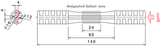
Figure 6. Specimen geometry and designated failure area.

Figure 7. Scheme of test set-up on a servo-hydraulic test rig.
strain-control. Hereby the strain signal from the extensometer is correlated to the displacement-signal of the machine. For test evaluation the stress-strain hysteresis is needed. Therefore, the stress as well as the strain is recorded throughout the entire test time. In addition the cylinder position and the temperature is recorded. To ensure a sufficient accuracy, the record-rate is at least 10 times higher than the highest test frequency. The highest frequencies occur at the lowest strain levels, that’s why at least a record-rate of 20 Hz is chosen for all tests. Data are stored continuosly over the whole test to get informations about all load cycles. These informations are exermined and reduced in a data processing-step after the test. A relatively long storage period, compared with high record-rates, lead to big amounts of data. The used machine-software, for whatever reasons, cannot relate the data points to load cycles, therefore this has to be done later.
3.3. Test Methodology
As mentioned in Section 2.1, a constant strain signal is used for loading. The extensometer is directly clipped on in the parallel middle part (see Figure 6) of the used sepcimen. To avoid effects, due to the strain rate dependent material behaviour and for better comparability to quasi-static tests, a constant strain rate of is chosen for testing. This is ensured by the use of a triangular instead of a sinusodial signal. With pretests the applicapility of this approach can be clarified and an influence of the load signal (e.g. harmonics) can be eliminated. By proceeding with a constant strain rate, the test frequencies depend on the given strain level following Equation (8). The factor 4 is needed to convert the periodic duration for one load flank (flanks marked in Figure 8 as light grey and grey lines). If the strain rate is given as , this must be captured by including 1/60.
(8)
The used strain amplitudes result in test frequencies of . At the beginning of each test the damage-free modulus is derived as a reference. To be able to determine , a stress controlled ramp is included in the test procedure as shown in Figure 8. To ensure a pure elastic response, a pressure load of is chosen. The modulus is derived from
the stress at this load-level and the measured strain. After a time of 10 s, the stress is reduced to zero and the strain controlled test starts. To describe the cyclic material behaviour in the LCF-regime of the S/N-curve strain levels where defined to achieve a range of cycles to failure from to . The total specimen separation or exceeding are used as abort criterions. At least one specimen is tested at each strain-level. Results are evaluated, according to [33].
3.4. Test Data Evaluation
The continous recorded stress and strain data are the basis for a comprehensive data evaluation. To get informations for each load cycle, raw data are splitted according to the load cycles. Therefore, the minima, the maxima as well as the mean crossings (zero-crossings in pure tension/compression) in the strain signal are evaluated. The stress and strain signal are then splitted into single sections and further combined to cycles. As soon as the minima and maxima of each loop are known, the reversal points can be calculated. The stiffness degradation over

Figure 8. Test procedure of strain controlled test.
the entire test is characterized by the elastic modulus E. Since polymer based materials show a non-linear material behaviour even on low load levels, the cyclic modulus is evaluated between two defined points. Following the evaluation of the secant modulus of quasi-static test, according to [34], a strain of and after the reversal points at and for each hysteresis is chosen. The modulus for the load path as well as the modulus for the unload path are evaluated this way. Additionally the tip modulus and the dynamic modulus acording to Equation (9) and (10) can be evaluated. [35] With these quantities, the influences of longterm effects during cyclic loading can be described. While the tip modulus decreases due to cyclic creep, the dynamic modulus stays at a constant level. A hysteretic heating and an progressing material damage lead to a hysteresis-tilt and have an influence on both muduli with proceeding cycle number. If hysteretic heating can be excluded, the different evolution of the tip modulus and the dynamic modulus allows the distinction between creep and material damage. In Figure 9 all evaluated data are shown for one hysteresis loop.
(9)
(10)
The enclosed hysteresis-area gives information about the stored and dissipated energy. Therefore the area is evaluated for each cycle according to Equation (11).
(11)
As all hysteresis loops are recorded, it’s easy to identify the last load cycle (number of cycles at failure) as well as some other interesting cycles, so that all other cylces can be deleted to reduce the amount of data. For the evaluation of low cycle fatigue data, the cycles at and are the most important.
Therefore, these cycles are stored. To record the effect of cyclic loads on the hysteresis additionally, the first two and one cycle per decade are stored.
Beside information to describe the single hysteresis, the number of cycles at break respectively and the corresponding strain- and stress-amplitude are necessary to describe the material behaviour in the LCF-regime. The cyclic stress/strain-curve is given by the corresponding amplitudes at for each strain level. To set up the -curve, the number of cycles to failure N is evaluated for each test. In Figure 5 the most important values are plotted. For each hysteresis the stress and strain must be evaluated at the reversal points. Based on this data, the models according to Equations (6) and (5) can be evaluated and the parameters (see Figure 5) can be derived.
4. Results
In Figure 10, the hysteresis loops for the first two, one intermediate and one of
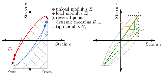
Figure 9. Evaluated hysteresis parameter.
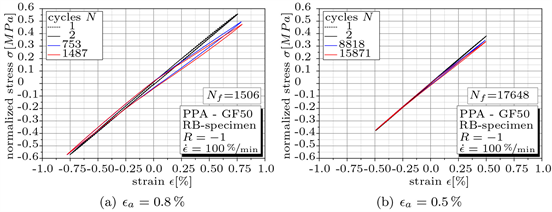
Figure 10. Hysteresis-loops for two strain levels.
the very last cycles, are plotted for the highest and lowest tested strain amplitude. The number of cycles at break is given for both tests. Just a small expansion of the hysteresis can be found even at the highest tested strain amplitude of . At the lowest level practically no expansion occurs. The expansion under tensile load is slightly more pronounced than under pressure. A small change in hysteresis-shape indicates a low amount of visco-elastic behaviour even at high strain amplitudes. The reduction of the maximum stress over the entire test remains on a low level. At break a total reduction of about 14% can be determined. This implies a very stiff material behaviour with a small amount of relaxation.
To distinguish between creep effects and mechanical damage the tip-modulus according Equation (9) and the dynamic modulus according Equation (10) are compared. If the averaged temperature (normalized by the initial temperature), measured at the specimen surface in the designated failure area (see Figure 6), doesn’t change significantly during the test, hysteretic heating can be excluded (dashed lines in Figure 11). Slight fluctuations and increase of temperature during the test stay under 3˚C. A change of temperature of 5˚C causes only a deviation in mechanical properties of 2% in the investigated temperature range (23˚C ± 5˚C) and therefore these fluctuations can be neglected. The difference between the two moduli represents the share of the mechanical damage on the total damage. In Figure 11 the curves for two strain-levels are plotted, in relation to the initial value. While the total damage at the higher strain-level is nearly evenly distributed between both damage modes, the mechanical damage is dominant at a low level. The pronounced share of mechanical damage up to high strain levels allows a stress based asessment.
To describe the cyclic material behaviour in the LCF-regime, tests have been performed with different strain-amplitudes. Based on the described test results, the stabilized -curve as well as the -curve (see Figure 5) can be described. In Table 1 the derived model parameters for both curves are summarized. For both curves the strain-amplitude and stress-amplitude determined at are used to derive the model parameters according to Equation (6), (5) and (7). In Figure 12(a) the stabilized -curve is shown. The curve shows, as mentioned before, a low amount of viscous strain. Plotting the strain-amplitude against the oscillation reversals, the -curve in Figure 12(b) is obtained.

Figure 11. Evaluation of the normalized tip-modulus , dynamic modulus and temperature T.
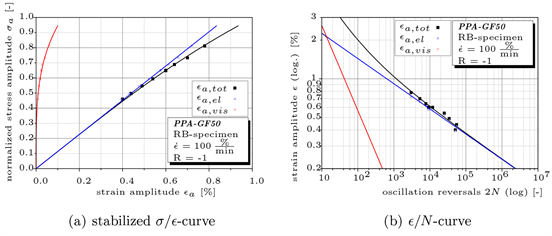
Figure 12. Test results to describe the LCF-regime.

Table 1. Derived model parameters from tests.
These two curves can be easily implemented in a data set [32] and enable the consideration of stress-rearrangement in a stress based lifetime assessment, according Figure 1, as well as a prediction following strain based approaches.
5. Discussion
With the conducted tests the applicability of strain controlled tests for highly filled fibre reinforced polymers is verified. To avoid influences due to the strain rate dependend material behaviour, a triangular loading signal should be used for testing. Hereby a constant strain rate can be ensured. Despite of low test frequencies small deviation between controll-signal and response-signal can occur, due to the discontinuity of a triangular signal. Therefore, a precise machine tunig is necessary to avoid influences coming from the load signal. As already metioned in the former section, just a small expansion of the hysteresis can be found even at the highest strain levels. This indicates a very small amount of visco-elastic deformations. A small temperature rise during the whole test, as shown in Figure 11, confirm this result, because visco-elastic deformation lead to a temperature rise, due to hysteretic heating. Benaarbian et al. show in [36] [37] the thermo-mechanical behaviour of a short E-glass fibre reinforced PA6.6 under different loading conditions. Tests at 1 Hz for highly oriented specimens show also very slender hysteresis and a small rise of temperature and therefore quite similar results compared to results shown in this work. Nevertheless, the higher fibre content of the investigated material lead to a stiffer material and by implication to lower visco-elastic deformation. A temperature rise at the end of specimen life time is induced by the ongoing damage and the correlated higher dissipation. Besides the temperature the comparison between tip— and dynamic modulus gives an idea about the shares of creep—and mechanical-damage. Zahnt describes in [35] the distinction of long time effects during cylic loading, so long as no hysteretic heating occur during the tests. Evaluating the two moduli following this method, the share of mechanical damage at is nearly 70% for all strain levels. The high amount of short fibres in the matrix leads to a pronounced share of mechanical damage in the material. The fibres act like inperfections within the matrix, so that initial cracks occur at the fibre ends. They propagate until they meet and form a macroscopic crack. [10] Mortazavian shows in [38] a similar behaviour for two fibre reinforced materials (PBT and PA6) under stress control. This suggests that a stress based lifetime assessment can be conducted up to high stress amplitudes for highly filled polymers. Nevertheless, the hysteresis shows a pronounced increase in strain during the tests because the maximum strain is not limited. This may lead to an overevaluation of the creep damage. Comparative investigations between stress and strain controlled tests on a fibre reinforced material in [39] show longer life times under strain control. To compare the tests with the same stress amplitude at were used. Especially for short number of load cycles , a pronounced difference (~50%) can be found. With an increasing number of cycles, the deviation is reduced continuously, so that the difference at N ~ 105 is under 20%. This can be attributed to a lower amount of creep damage. For smaller filling grades, the influence of the visco-elastic matrix increases. This leads to a higher proportion of the creep component, so that less or unreinforced materials may be can not be tested this way. As shown in Figure 12, a nearly linear relation can be found for the stabilized -curve Figure 12(a) as well as for -curve Figure 12(b). From this two curves the parameter of Equation (5) and (6) are derived and summarized in Table 1. While the parameters b and c are mainly within the range of metals the strain hardening coefficient n differs. Abood shows in [40] comparable results for unreinforced materials. The visco-elastic material behaviour of polymers instead of a plastic material behaviour requires further investigations and new models to describe the “strain hardening” effect. In principle both methods strain- or stress-controlled tests can be used to describe the material behaviour in the low cycle fatigue regime. Due to a higher amount of creep-damage, stress controlled tests may lead to an underestimation of the lifetime. With the shown tests the material behaviour of the investigated material can be determined in the LCF-regime of the S/N-curve. With the cyclic stabilized -curve the stress rearrangement according to Neuber can be implemented in the life time assessment, based on local stresses. Further the -curve enables a strain based lifetime assessment. Nevertheless, additionally studies have to be done to clarify the general applicability and influences such as fibre orientation, temperature and mean-strain.
6. Summary and Outlook
To describe the fatigue behaviour of a short fibre reinforced material in the low cycle regime of the S/N-curve, strain controlled tests were performed. For each hysteresis loop the maximum and minimum stress and strain are determined. In addition to the tension-, compression- as well as the dynamic- and the tip-modulus are derived to describe the stiffness reduction. The comparison of the dynamic- and the tip-modulus gives information about the shares of damage on the total damage. Based on the test results, the cyclic stabilized -curve as well as the -curve are derived and implemented in a dataset for the lifetime assessment. With the described procedure, with strain controlled tests, the fatigue life time of reinforced polymers in the low cycle regime of the S/N-curve can be described. To clarify the influence between stress and strain control, further tests must be conducted at equivalent load levels. The behaviour of reinforced polymers strongly depends on the amount of reinforcement, their orientation, surrounding temperature and counting other effects. Therefore the most important effects have to be identified and tests have to be performed to describe them. The use of unified material laws, well known for metals, should be examined.
Acknowledgements
The research work of this paper was performed at the Department of Product Engineering at the Montanuniversität Leoben in collaboration with the Polymer Competence Center Leoben GmbH (PCCL, Austria) within the framework of the COMET-program of the Austrian Ministry of Traffic, Innovation and Technology with contribution by BMW-Group, Robert Bosch GmbH, Engineering Center Steyr (MAGNA Powertrain ECS), EMS-Grivory, VW-Group, Schaeffler Technologies AG & Co KG and Qualitech AG. The PCCL is founded by the Austrian Government and the State Governments of Styria, Lower and Upper Austria.
Conflicts of Interest
The authors declare no conflicts of interest regarding the publication of this paper.
Cite this paper
Primetzhofer, A., Stadler, G., Pinter, G. and Grün, F. (2019) Applicability of Strain Controlled Cyclic Tests for Short Fibre Reinforced Polymers. Materials Sciences and Applications, 10, 568-583. https://doi.org/10.4236/msa.2019.108041
References
- 1. Haibach, E. (2006) Betriebsfestigkeit: Verfahren und Daten zur Bauteil-berechnung, VDI-Buch. Springer, Berlin. https://doi.org/10.1007/3-540-29364-7
- 2. Radaj, D. and Vormwald, M. (2007) Ermüdungsfestigkeit: Grundlagen für Ingenieure. 3rd Edition, Springer, Berlin. https://doi.org/10.1007/978-3-540-71459-0
- 3. Primetzhofer, A., Stadler, G., Pinter, G. and Grün, F. (2019) Lifetime Assessment of Anisotropic Materials by the Example Short Fibre Reinforced Plastic. International Journal of Fatigue, 120, 294-302. https://doi.org/10.1016/j.ijfatigue.2018.06.013
- 4. Unger, B., Fleischer, H., Guster, C. and Pinter, G. (2008) Lebensdauerberechnung für kunststoff komponenten. In: DVM, Eds., DVM-Tag 2008 Leichtbaustrategien, Vol. 675, DVM, Berlin, 39-51.
- 5. Fleischer, H., Brune, M., Thornagel, M., Thomas, B. and Guster, C. (2009) Von derspritzgie simulation zur betriebsfestigkeitsdimensionierung—entwicklung und einsatz einer durchgängigen simulationskette. Kunststoffe im Automobilbau, 1-23.
- 6. Guster, C., Pinter, G., Mösenbacher, A. and Eichlseder, W. (2011) Evaluation of a Simulation Process for Fatigue Life Calculation of Short Fibre Reinforced Plastic Components. Procedia Engineering, 10, 2104-2109. https://doi.org/10.1016/j.proeng.2011.04.348
- 7. Eriksson, A. (2003) Fatigue of Injection Moulded Short Fibre Reinforced Polymers. PhD Thesis.
- 8. Guster, C., Friesenbichler, W. and Gröger, T. (2013) Simulating the Fatigue Life of Fibre Reinforced Injection Moldings. Kunststoffe, 9, 92-94.
- 9. Mösenbacher, A., Brunbauer, J., Pichler, P.F., Guster, C. and Pinter, G. (2014) Modeling and Validation of Fatigue Life Calculation Method for Short Fibre Reinforced Injection Moulded Parts. 16th European Conference of Composite Materials, Seville, 22-26 June 2014, 1-8.
- 10. Ansari, M.T.A., Singh, K.K. and Azam, M.S. (2018) Fatigue Damage Analysis of Fiber-Reinforced Polymer Composites: A Review. Journal of Reinforced Plastics and Composites, 37, 636-654. https://doi.org/10.1177/0731684418754713
- 11. Guedes, R.M. (2019) Lifetime Prediction of Polymers and Polymer Matrix Composite Structures: Failure Criteria and Accelerated Characterization. In: Creep and Fatigue in Polymer Matrix Composites, Elsevier, Amsterdam, 269-301. https://doi.org/10.1016/B978-0-08-102601-4.00009-6
- 12. Hirschberg, V., Lacroix, F., Wilhelm, M. and Rodrigue, D. (2019) Fatigue Analysis of Brittle Polymers via Fourier Transform of the Stress. Mechanics of Materials, 137, Article ID: 103100. https://doi.org/10.1016/j.mechmat.2019.103100
- 13. Kim, H.S. (2019) S-n Curve and Fatigue Damage for Practicality. In: Creep and Fatigue in Polymer Matrix Composites, Elsevier, Amsterdam, 439-463. https://doi.org/10.1016/B978-0-08-102601-4.00014-X
- 14. Lee, C.S., Kim, H.J., Amanov, A., Choo, J.H., Kim, Y.K. and Cho, I.S. (2019) Investigation on Very High Cycle Fatigue of PA66-GF30 GFRP Based on Fiber Orientation. Composites Science and Technology, 180, 94-100. https://doi.org/10.1016/j.compscitech.2019.05.021
- 15. Sevenois, R.D.B. and van Paepegem, W. (2019) Fatigue Testing for Polymer Matrix Composites. In: Creep and Fatigue in Polymer Matrix Composites, Elsevier, Amsterdam, 403-437. https://doi.org/10.1016/B978-0-08-102601-4.00013-8
- 16. Bernasconi, A., Davoli, P., Basile, A. and Filippi, A. (2007) Effect of Fibre Orientation on the Fatigue Behaviour of a Short Glass Fibre Reinforced Polyamide-6. International Journal of Fatigue, 29, 199-208. https://doi.org/10.1016/j.ijfatigue.2006.04.001
- 17. Guster, C., Pinter, G., Lang, R.W., Eichlseder, W. and Balika, W. (2008) Fiber Orientation and Fatigue Behavior of a Short Glass-Fiber Reinforced Partial Aromatic Polyamide. In: Chair of Mechanical Engineering, Eds., 2nd Fatigue Symposium Leoben, Chair of Mechanical Engineering, Leoben, 444-456.
- 18. Brunbauer, J., Mösenbacher, A., Guster, C. and Pinter, G. (2014) Fundamental Influences on Quasistatic and Cyclic Material Behavior of Short Glass Fiber Reinforced Polyamide Illustrated on Microscopic Scale. Journal of Applied Polymer Science, 131. https://doi.org/10.1002/app.40842
- 19. Nienhaus, R. and Kurzbeck, S. (2014) Influence of Notches on the Fatigue Behaviour of Short Fibre Reinforced Polyamide Considering Environmental Temperature. 16th European Conference of Composite, Seville, 22-26 June 2014, 1-8.
- 20. Lüders, C., Krause, D. and Kreikemeier, J. (2018) Fatigue Damage Model for Fibre Reinforced Polymers at Different Temperatures Considering Stress Ratio Effects. Journal of Composite Materials, 52, 4023-4050. https://doi.org/10.1177/0021998318773466
- 21. Mösenbacher, A., Guster, C., Pinter, G. and Eichlseder, W. (2012) Investigation of Concepts Describing the Influence of Stress Concentration on the Fatigue Behavior of Short Glass Fibre Reinforced Polyamide. European Conference of Composite Materials, Venice, 24-28 June 2012.
- 22. Mallick, P.K. and Zhou, Y. (2004) Effect of Mean Stress on the Stress-Controlled Fatigue of a Short e-Glass Fiber Reinforced Polyamide-6,6. International Journal of Fatigue, 26, 941-946. https://doi.org/10.1016/j.ijfatigue.2004.02.003
- 23. Primetzhofer, A., Mõsenbacher, A. and Pinter, G. (2015) Influence of Mean Stress and Weld Lines on the Fatigue Behaviour of Short Fibre Reinforced Polyamide. 20th International Conference on Composite Materials, Copenhagen, 19-24 July 2015.
- 24. Lu, Z., Feng, B. and Loh, C. (2018) Fatigue Behaviour and Mean Stress Effect of Thermoplastic Polymers and Composites. Frattura ed Integrità Strutturale, 12, 150-157. https://doi.org/10.3221/IGF-ESIS.46.15
- 25. Neuber, H. (1961) Theory of Stress Concentration for Shear-Strained Prismatical Bodies with Arbitrary Nonlinear Stress-Strain Law. Journal of Applied Mechanics, 28, 544-550. https://doi.org/10.1115/1.3641780
- 26. Ramberg, W. and Osgood, W.R. (1943) Description of Stress-Strain Curves by Three Parameters. Technical Note No. 902, National Advisory Committee for Aeronautics, Washington DC.
- 27. Manson, S.S. (1965) Fatigue: A Complex Subject: Some Simple Approximations. Experimental Mechanics, 5, 193-226. https://doi.org/10.1007/BF02321056
- 28. Coffin, L.F. (1954) A Study of the Effects of Cyclic Thermal Stresses on a Ductile Metal. Transactions of the ASME, 76, 931-950.
- 29. Morrow, J. (1965) Cyclic Plastic Strain Energy and Fatigue of Metals. In: Lazan, B.J., Ed., Internal Friction, Damping, and Cyclic Plasticity, American Society for Testing & Materials, West Conshohocken, 45. https://doi.org/10.1520/STP43764S
- 30. Mösenbacher, A. and Guster, C. (2012) Fatigue Behaviour of a Short Glass Fibre Reinforced Polyamide: Effect of Notches and Temperature. 3nd Fatigue Symposium, Leoben, 152-160.
- 31. Primetzhofer, A., Stadler, G., Pinter, G. and Grün, F. (2018) Implementation of Variable Amplitude Tests in Life Time Assessment of Short Fibre Reinforced Polymers. 7th International Conference on Fatigue of Composites, Vicenza, 4-6 July 2018.
- 32. Primetzhofer, A., Stadler, G., Pinter, G. and Grün, F. (2019) Data Set Determination for Lifetime Assessment of Short Fibre Reinforced Polymers. Zeitschrift Kunststofftechnik: Journal of Plastics Technology, 15, 26.
- 33. ASTM (2010) Practice for Statistical Analysis of Linear or Linearized Stress-Life (S-N) and Strain-Life (ε-N) Fatigue Data. https://doi.org/10.1520/E0739-10
- 34. Grellmann, W., Seidler, S. and Alstädt, V. (2013) Polymer Testing, 2nd Edition, Hanser Publishers, Munich. https://doi.org/10.3139/9781569905494
- 35. Zahnt, B.A. (2003) Ermüdungsverhalten von diskontinuierlich glasfaserverstärkten kunststoffen. Dissertation, Montanuniversität Leoben, Leoben.
- 36. Benaarbia, A., Chrysochoos, A. and Robert, G. (2015) Fiber Orientation Effects on Heat Source Distribution in Reinforced Polyamide 6.6 Subjected to Low Cycle Fatigue. Journal of Engineering Mathematics, 90, 13-36. https://doi.org/10.1007/s10665-014-9720-7
- 37. Benaarbia, A., Chrysochoos, A. and Robert, G. (2015) Thermomechanical Behavior of PA6.6 Composites Subjected to Low Cycle Fatigue. Composites Part B: Engineering, 76, 52-64. https://doi.org/10.1016/j.compositesb.2015.02.011
- 38. Mortazavian, S. and Fatemi, A. (2015) Fatigue Behavior and Modeling of Short Fir Reinforced Polymer Composites Including Anisotropy and Temperature Effects. International Journal of Fatigue, 77, 12-17. https://doi.org/10.1016/j.ijfatigue.2015.02.020
- 39. Mösenbacher, A. (2014) Modellentwicklungen zur betriebsfesten auslegung von strukturbauteilen aus glasfaserverstärkten thermoplasten im motorraum. Dissertation, Montanuniversität Leoben, Leoben.
- 40. Abood, A.N., Saleh, A.H., Ali, A.A. and Humood, L.K. (2011) Low Cycle Fatigue of Different Polymer Types PA, PVC and POM. Mechanical Engineering, 38, 4154-4156.