Journal of Modern Physics
Vol.08 No.11(2017), Article ID:79808,14 pages
10.4236/jmp.2017.811107
Carnot Factor of a Vapour Power Cycle with Regenerative Extraction
Duparquet Alain
Engineering Energy Equipment, Bourgoin-Jallieu, France

Copyright © 2017 by author and Scientific Research Publishing Inc.
This work is licensed under the Creative Commons Attribution International License (CC BY 4.0).
http://creativecommons.org/licenses/by/4.0/


Received: September 14, 2017; Accepted: October 21, 2017; Published: October 24, 2017
ABSTRACT
The present paper describes the energy analysis of a regenerative vapour power system. The regenerative steam turbines based on the Rankine cycle and comprised of vapour extractions have been used industrially since the beginning of the 20th century, particularly regarding the processes of electrical production. After having performed worked in the first stages of the turbine, part of the vapour is directed toward a regenerative exchanger and heats feedwater coming from the condenser. This process is known as regeneration, and the heat exchanger where the heat is transferred from steam is called a regenerator (or a feedwater heater). The profit in the output brought by regenerative rakings is primarily enabled by the lack of exchange of the tapped vapour reheating water with the low-temperature reservoir. The economic optimum is often fixed at seven extractions. One knows the Carnot relation, which is the best possible theoretical yield of a dual-temperature cycle; in a Carnot cycle, one makes the assumption that both compressions and expansions are isentropic. This article studies an ideal theoretical machine comprised of vapour extractions in which each cycle partial of tapped vapour obeys these same compressions and isentropic expansions.
Keywords:
Thermodynamic, Carnot Factor, Rankine Cycle, Power Plant, Energy, Efficiency, Entropy, Second Law Analysis, Irreversibility, Regenerative Cycle, Thermal Cycle

1. Introduction
The work output is maximised when the process between the two specified states is executed in a reversible manner. However, according to the second law of thermodynamics, such a reversible process is not possible in practice. A system delivers the maximum possible work as it undergoes a reversible process from the specified initial state to the state of its environment, that is, the dead state.
According with M.Pandey, T.K Gogoi [1] , the study of thermodynamic cycles applied to power stations is of great importance due to the increasing energy consumption, the opening of electricity markets and the increasingly strict environmental restrictions (specifically regarding the carbon dioxide emissions issue). Power plants that use steam as their working fluid operate on the basis of the Rankine cycle (1). The first stage in designing these power plants is performing the thermodynamic analysis of the Rankine cycle.
According with Da Cunha, A., Fraidenraich, N. and Silva, [2] and Baumann, K., [3] , the regenerative cycle is a modified Rankine cycle which intends to improve the efficiency of the system. Baumann (1930) analyzed the development of steam cycle power during years, using high steam pressure and temperature, with the objective to improve the efficiency of the power plants. There are some advantages of regenerative power cycle compared of Rankine cycle. The thermal stresses in the collectors are minimized because of the water being hotter. The steam condenser size can be reduced, the pumps energy to cool the steam condenser is reduced in the same proportion. But also there are some disadvantages as the plant become more complicated, more expensive and increase the number of maintenance. Many industries use steam based thermodynamic cycles. Water steam is generated in a boiler, which brings the steam to a high pressure and a high temperature. The steam expands in a turbine to produce work. The steam then passes through a condenser. In this cycle, referred to as the Rankine or Hirn cycle, the heat referred to as “waste” is the heat exchanged in the condenser.
A regenerative cycle is a cycle in which part of the waste heat is used for heating the heat-transfer fluid. Since the early 20th century, steam turbines have been most frequently used in regenerative cycles, e.g., in thermal and nuclear power plants. These steam engines are equipped with five to seven steam extractions. Part of the steam that performed work in the turbine is drawn off for use in heating the water. Regeneration or the heating up of the feedwater by the steam extracted from the turbine has a marked effect on the cycle efficiency. Figure 1 presents diagram of a regenerative steam extraction.
The mass of steam generated for the given flow rate of flue gases is determined by the energy balance. In fact, the drawn-off steam is proportional to the flow of water to be heated to conserve both mass and energy.
2. Simple Rankine Cycle
2.1. Real Cycle
The thermodynamics first principle stipulates that over a cycle, .
(1)
(2)
(3)

Figure 1. Diagram of a regenerative steam extraction cycle.
where,
= mass enthalpy of the high-temperature reservoir.
= mass enthalpy of the low-temperature reservoir.
The transferred energy is equal to the differential specific enthalpy multiplied by the fluid mass
(4)
The energy efficiency of the engine power is defined as
(5)
The efficiency is rewritten using (1), (3) and (5) as follows:
(6)
The following is deduced from (4) and (6):
(7)
(8)
where:
= fluid mass.
= specific enthalpy of the hot vapour to the admission of the turbine.
= specific enthalpy in liquid form.
= specific enthalpy of the cold vapour to the exhaust of the turbine.
Figure 2 presents the real Rankine cycle in T-s diagram.
The cycle performance is deduced from (5)-(8) as
(9)
2.2. Ideal Carnot Cycle
Let us consider now that the cycle is performed with ideally isentropic com-

Figure 2. The real Rankine cycle (shown in red).
pressions and isentropic expansions.
According with Lucien Borel [4] , the heat exchanged with the high-temperature reservoir is equal to
(10)
where
= temperature of the high-temperature reservoir.
= cold vapour specific entropy to the exhaust of the turbine.
= cold condensate water specific entropy.
Figure 3 presents the real Rankine cycle in T-s diagram in red en the coloured surface corresponds to the total energy of a high-temperature reservoir that would be necessary if the cycle obeyed the assumptions of isentropic compressions and isentropic expansions (10).
The heat exchanged with the low-temperature reservoir is equal to
(11)
where = temperature of the low-temperature reservoir.
Figure 4 presents the Real cycle in red. The coloured surface corresponds to the total energy of low-temperature reservoir that would be necessary if the cycle

Figure 3. The real cycle is represented in red. The coloured surface corresponds to the total energy of a high-temperature reservoir that would be necessary if the cycle obeyed the assumptions of isentropic compressions and isentropic expansions (10).
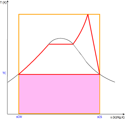
Figure 4. The Real cycle is represented in red. The coloured surface corresponds to the total energy of low-temperature reservoir that would be necessary if the cycle obeyed the assumptions of isentropic compressions and expansions (11).
obeyed the assumptions of isentropic compressions and expansions (11).
The cycle efficiency is deduced from (6), (10) and (11) as
(12)
which is equal to the Carnot factor.
(13)
3. Thermodynamics Analysis of Steam Power Cycle with One Feed Waterheater
3.1. Real Cycle with One Feedwater Heater
We study here the evaluation of the output of a cycle comprised of only 1 steam extraction.
To determine the output of the cycle comprising an extraction, we separate this cycle into 2 partial cycles.
The heat of the hot reservoir in the cycle is equal to the sum of the heat of the hot reservoir of the principal cycle and the heat of hot reservoir of the cycle partial of the extraction vapour:
The heat of hot reservoir of the principal cycle is equal to (7).
The heat of hot reservoir of the cycle partial of the extraction vapour is equal to
(14)
where
= enthalpy of the hot reservoir of the cycle partial of extraction.
= extraction vapour mass.
= extracted steam specific enthalpy in liquid form.
One form of the deduced total heat from the hot reservoir:
(15)
where
= vapour mass exchanging with the low-temperature reservoir in the condenser
The heat of the low-temperature reservoir in the cycle is equal to the sum of the heat of the low-temperature reservoir of the principal cycle and the heat of the low-temperature reservoir of the partial cycle of the tapped vapour:
The heat of low-temperature reservoir of the principal cycle is equal to (8)
The heat of low-temperature reservoir of the cycle partial of the tapped vapour is equal to:
(16)
where
= enthalpy of the low-temperature reservoir of the partial cycle of extraction
= the mass vapour enthalpy harnessed by the extraction side.
One form of the deduced total heat from the low-temperature reservoir:
(17)
The cycle efficiency is deduced from (6), (15) and (17)
(18)
The output of a regenerative cycle comprising an extraction is clearly higher than that of a non-regenerative simple cycle. It is enough to compare the expressions of the output in (18) and in (9).
The mass of the steam generated for the given flow rate of flue gases, mex, is obtained from the energy balance.
Heat gained by the steam = Heat lost by the flue gases.
(19)
Figure 5 presents the cycle represented in red is the principal cycle traversed

Figure 5. The cycle represented in red is the principal cycle traversed by the vapour mass “m”. The cycle represented in blue is the cycle traversed by the mass “mex” of the tapped vapour.
by the vapour mass “m”. The cycle represented in blue is the cycle traversed by the mass “mex ”of the tapped vapour.
3.2. Ideal Cycle Comprised of One Feedwater Heater
Let us now consider that the two cycles are ideally performed via compressions and expansions that are isentropic.
Let us separate the cycles into two partial cycles.
The heat of the hot reservoir in the cycle is equal to the sum of the heat of the hot reservoir of the principal cycle and the heat of the hot reservoir of the partial cycle of the tapped vapour:
The heat of hot reservoir of the principal cycle is equal to (10).
Figure 6 presents the real principal cycle traversed by the vapour “m” mass is represented in red. The coloured surface corresponds to the total energy of the hot reservoir that would be necessary if the cycle obeyed the assumptions of isentropic compressions and isentropic expansions (10).

Figure 6. The real principal cycle traversed by the vapour “m” mass is represented in red. The coloured surface corresponds to the total energy of the hot reservoir that would be necessary if the cycle obeyed the assumptions of isentropic compressions and isentropic expansions (10).
(20)
Figure 7 presents the cycle represented in blue the real cycle traversed by the mass “mex” of the tapped vapour. The coloured surface corresponds to the total energy of the hot reservoir that would be necessary if the 2 cycles obeyed the assumptions of isentropic expansions and isentropic compressions (20).
One deduces the total heat from the hot reservoir as follows:
(21)
The heat of the low-temperature reservoir in the cycle is equal to the sum of the heat of the low-temperature reservoir of the principal cycle and the heat of the low-temperature reservoir of the partial cycle of the tapped vapour:
The heat of the low-temperature reservoir of the principal cycle is equal to (11).
Figure 8 presents the cycles in T-s diagram. The cycle represented in red is

Figure 7. The cycle represented in blue is the real cycle traversed by the mass “mex”of the tapped vapour. The coloured surface corresponds to the total energy of the hot reservoir that would be necessary if the 2 cycles obeyed the assumptions of isentropic expansions and isentropic compressions (20).
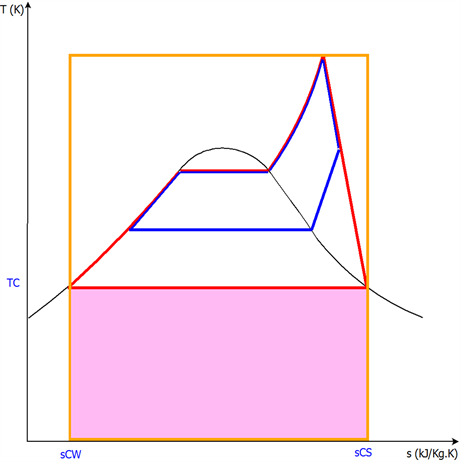
Figure 8. The cycle represented in red is the real cycle traversed by the mass “m” of the vapour. The coloured surface corresponds to the total energy of the low-temperature reservoir that would be necessary if the 2 cycles obeyed the assumptions of isentropic compressions and isentropic expansions.
the real cycle traversed by the mass “m” of the vapour.
The coloured surface corresponds to the total energy of the low-temperature reservoir that would be necessary if the 2 cycles obeyed the assumptions of isentropic compressions and isentropic expansions.
The heat of the low-temperature reservoir of the extracted steam partial cycle is equal to:
(22)
Figure 9 presents the cycles in T-s diagram. The heat of the low-temperature reservoir of the partial cycle of extraction is represented by the coloured surface. Note that the difference in entropy mass s is equal to the difference between the mass entropy of the cold vapour and the mass entropy of condensate of the principal cycle.
(23)
The energy efficiency is deduced from (6), (22), and (23):

Figure 9. The heat of the low-temperature reservoir of the partial cycle of extraction is represented by the coloured surface. Note that the difference in entropy mass s is equal to the difference between the mass entropy of the cold vapour and the mass entropy of condensate of the principal cycle.
which can be expressed as:
(24)
Applying Equation (19), one determines the mex mass value according to the m mass:
(25)
(26)
4. Generalised Thermodynamics Analysis of a Steam Power Cycle with “N” Number of Feedwater Heaters
4.1. Real Cycle with Two Feedwater Heaters
The thermodynamic cycles of steam turbines are comprised of between five and eight extractions. We treat here the case of a machine comprised of two extractions; this methodology can be extended to account for a higher number of extractions. The output is deduced from (18)
(27)
where:
= vapour mass of the first extraction. (Recall that the classification numbering of conventional feedwater heaters starts from the condenser.)
= specific enthalpy of the steam that heats feedwater heater number 1.
= mass of condensate from extraction number 2.
= specific enthalpy of extraction number 1 vapour.
= specific enthalpy of the condensed water into feedwater heater number 1.
= specific enthalpy of extraction number 2 vapour.
Calculation of
One deduces from (19)
(28)
4.2. Ideal Cycle “n” Number of Feed Water Heaters
One deduces the output from the ideal cycle from (30) and (26):
(29)
where:
= temperature of the condensate with extraction vapour number 1
= temperature of the condensate with extraction vapour number 2
One generalises the following:
(30)
One deduces from (26) and (28)
(31)
One deduces from (29) and (31) the following:
(32)
The above result (32) can be generalised as follows:
(33)
5. Conclusions
The Carnot factor, as is universally known, is a typical case limited to the cycles that do not involve feedwater heaters. In the case of regenerative cycles, the Carnot factor of a machine is given by the following relationship:
This relationship obeys the second principle of thermodynamics: the variation of the entropy of an unspecified thermodynamic system, due to the internal operations, can be only positive or worthless.
Whatever the fluid, if it is possible to use a part of its mass and not to exchange with the low-temperature reservoir, it is advantageous. An example to consider the following issue is about combined cycles. A part of designers of electrical generating units using the combined cycles of a gas turbine and a steam turbine do not use the regenerative Rankine cycle. This is because they consider that they have achieved a yield close to Carnot’s performance. This article demonstrates that it is irrelevant. The advantage in this case is above all to reduce the steam condenser size. The pumps energy to cool the steam condenser is reduced in the same proportion. If an atmospheric refrigerant is used, the economy would be significant.
Cite this paper
Alain, D. (2017) Carnot Factor of a Vapour Power Cycle with Regenerative Extraction. Journal of Modern Physics, 8, 1795-1808. https://doi.org/10.4236/jmp.2017.811107
References
- 1. Pandey, M. and Gogoi, T.K. (2013) International Journal of Emerging Technology and Advanced Engineering, 3, 427-434.
- 2. Da Cunha, A., Fraidenraich, N. and Silva, L. (2017) Journal of Power and Energy Engineering, 5, 45-55. https://doi.org/10.4236/jpee.2017.58004
- 3. Baumann, K. (1930) Proceedings of the Institution of Mechanical Engineers, 2, 1305. https://doi.org/10.1243/PIME_PROC_1930_119_024_02
- 4. Borel, L. Thermodynamique et énergétique. [Thermodynamics and Energetics.] presses polytechniques et universitaires Romandes 3ème édition revue et corrigée ISBN 2-88074-214-5 CH 1015 Lausanne.
Nomenclature
T Temperature (K)
s Specific Entropy (J/kg∙K)
P Pressure (Pa)
h Specific Enthalpy (J/kg)
W Work (J)
Q Heat (J)
H Enthalpy (J)
Main Steam Cycle Mass (kg)
Extraction Steam Feedwater Mass (kg)
Extraction Steam Feedwater Number 1 Mass (kg)
Extraction Steam Feedwater Number 2 Mass (kg)
Energy Efficiency (%)
Sum
Product
Integral