Journal of Modern Physics
Vol.07 No.01(2016), Article ID:62621,8 pages
10.4236/jmp.2016.71005
Hierarchic Computations in Geometric Space―Showing Sharp Diffraction in Quasicrystals
Antony J. Bourdillon
UHRL, San Jose, CA, USA

Copyright © 2016 by author and Scientific Research Publishing Inc.
This work is licensed under the Creative Commons Attribution International License (CC BY).
http://creativecommons.org/licenses/by/4.0/


Received 7 December 2015; accepted 5 January 2016; published 8 January 2016
ABSTRACT
A quasi-structure factor method is used to show how sharp diffraction patterns are produced by aperiodic quasicrystals. Icosahedral symmetry is described for the tensor rank 3 solids with edge- sharing unit cells that are pentagonally close packed in hierarchic structures having a geometric reciprocal lattice. The hierarchic symmetry replaces translational symmetry in crystal diffraction. Details in the calculation show how the symmetry is simulated in diffraction.
Keywords:
Quasicrystals, Geometric Space, Structure Factors, Scattering Factors, Hierarchic

1. Introduction
It is comparatively easy to represent, diagrammatically, structures such as nearly free electron energy bands in quasicrystals [1] , wave vector dispersion curves [2] , two dimensional tiling [3] , etc., all of which occur in geometric space [4] - [6] . Here we show how they are underpinned by detailed computations of quasi-structure-fac- tors that we use to understand diffraction in icosahedral quasicrystals. The first detail to be solved is the metric that must be used (not wrongly guessed1 [7] - [9] ) to interpret structural dimensions from experimental diffraction data. The problem is due to the fact that while the X-ray or electron probe is periodic in translation along their directions of propagation, the quasicrystal is an aperiodic scatterer. A way must therefore be found that accounts for the interaction between probe and specimen. The interaction is not Bragg diffraction since that law is valid only for crystals that are periodic, both in angular symmetry and in translational symmetry. Bragg diffraction is in linear order n, whereas the diffraction from quasicrystals is geometric. The quasicrystal has angular and hierarchic symmetries (i.e. lacking translational symmetry) with a geometric reciprocal lattice. In the quasicrystal, large calculations are limited by truncation errors required by multiple additions from the aperiodic structures. Shorter calculations lack precision [10] [11] , but a method that uses geometric quasi-scattering-factors [12] acts to both reduce the computation and increase the precision. In this paper the method is explained in detail for hierarchic structures.
Previously we have shown [1] [13] that icosahedral quasicrystals are pentagonal close packed, ideally on a hierarchic lattice. All of the structure, the diffraction pattern, the stereogram of principal axes, and the diffraction planes are described by rank 3 tensors in geometric space. The unit cell is extremely dense due to the precise ratio, DMn/DAl, between atomic diameter on the central solute atom and peripheral solvent atoms. The closest crystalline approximant to the quasicrystal is the matrix phase of melt spun Al6Mn, namely the face centered cubic (fcc) structure [14] .
The quasicrystal structure bridges the difference between crystal structures and compound amorphous materials such as fused silica. They all have unit cells. In crystals the cells fill space by face sharing on fourteen Bravais lattices. Their diffraction is sharp and it obeys Bragg’s law. The pattern shows linear order, n = 0, 1, 2, 3, 4… In compound glasses, unit cells are more or less randomly oriented and, typically, edge-sharing. The diffraction is correspondingly diffuse while being structured on Bragg’s law. Patterns are circular, though broader than patterns from polycrystalline specimens where greater radial sharpness resembles the point sharpness from crystals. Linear Bragg orders are again observed. In quasicrystals the diffraction patterns are sharp but not associated with any of the Bravais lattices. The order sequence is no longer linear but in geometric series, τm with integral . Stereograms [13] correspond to the icosahedral structure’s angular symmetry, as found in the experimental data from Al6Mn [15] . The unit cells are edge-sharing in a hierarchic structure with geometric period τ2, which is the stretching factor in cluster and supercluster orders. This arrangement has been observed in phase contrast microscopy [8] [16] . The phase contrast maps the heavy solute atom and its surrounding dense unit cell. In the experimental data, the diffraction peaks are so sharp [10] that the coherence demands unique explanation, especially because the quasicrystal is aperiodic.
The rank 3 ordering has been previously demonstrated and all diffracted beams in Shechtman’s data have been indexed and simulated [17] . Indexation follows the quasi-Bragg law , where m is the geometric order, and θ’ = cs∙θ is the quasi-Bragg angle. In case of small angles (θ << 1), as in transmission electron microscopy,

where for quasi-Miller indices h, k, l, . This compromise interplanar spacing in ico-
sahedral units2, is again different from the corresponding periodic interplanar spacing in Bragg diffraction. In quasicrystals, d’ measures not a single spacing periodically repeated; but the set of interplanar spacings in series τm. The law describes the structural aperiodicity that causes geometric radial symmetry in the diffraction pattern with icosahedral angular symmetry. With this law, simulated intensities match experimental values very well indeed. The only variable common to the Bragg law for crystals is λ. Likewise, derived interplanar spacings match phase contrast electron microscopy [8] , though the spacings have to be interpreted by means of a simulated metric that is consistent with compromise scattering by multiple planes in the aperiodic solids. The outstanding problem remains: how does an aperiodic solid produce a sharp diffraction pattern?
2. Quasi-Scattering Factors (QScF)
In quasicrystals these are adapted from crystals, where they are used for several purposes. The simplest is for the determination of allowed and forbidden diffraction lines in specific reciprocal lattices. These can be determined by relatively simple calculations on the unit cell when its structure is known. By contrast in quasicrystals, the primary use of structure factors lies in calculating the widely varying intensities that are seen in the diffraction patterns, due not to secondary aspects such as temperature, orientation, crystal size, etc., but due to intrinsic excitation of incident beams. Because the hierarchic structure lacks translational periodicity, the calculations must be made, not over the unit cell, but over the whole crystal. Since this is ideally infinite, a finite computation requires truncation of the ideal structure.
As in crystals, considerable simplification results from the fact that the icosahedral hierarchic structure is centro-symmetric. Scattering of an incident beam may therefore be calculated with real numbers contained in the cosine term, since the imaginary parts cancel. The structure factor Fhkl for a beam with indices h, k, l is then written [18] :
 (1)
(1)
summed over the N atoms in the unit cell, each with its specific scattering factor fi, in this case appropriate to either Al or Mn. Values can be found in various tables [19] . The coordinates x, y, z represent the locations of the atoms in the cell, as fractions of the unit cell lattice parameters. For the icosahedral structure, atomic sites are conveniently represented on Euclidean coordinates.
In adapting the formula to quasicrystals, three changes are made. Firstly, the basis cell used in measurement is taken to be the unit cube since the length to edge-width ratio of the icosahedron forms a golden rectangle [20] with dimensions τ × 1. The unit edge width is the diameter of the Al atoms. Secondly the summation is made over a conveniently selected truncation of the infinite ideal quasicrystal. Thirdly, because there is no reason to suppose that the diffraction follows Bragg’s law, an extra variable cs, the compromise spacing effect, is added as a factor beside fn. By scanning cs, and summing systematically at appropriate intervals, a clear maximum is found in the structure factor. The simulated value is cs = 0.947 (Figure 1), with the condition that the diffraction is understood as linear Bragg order n = 2 [6] [10] [12] , where orders 1, 3, 4, 5 etc. are suppressed in the geometric diffraction. This value for n is, like cs, a simulated maximum.
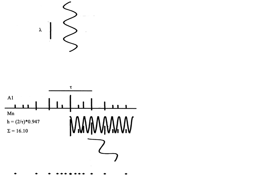
Figure 1. A periodic electron beam, moving downwards, scatters from atomic planes on an aperiodic quasicrystal cluster to form a diffraction pattern in geometric space. This is due to a Bloch wave having maximum overlap with the populations on the atomic planes [2] . Al atoms lie above the abscissa; Mn atoms below. The maximum overlap occurs at the quasi-Bragg angle cs∙θ, where θ would be the crystalline Bragg angle for diffraction from a corresponding unique interplanar spacing.
The suppression of higher Bragg orders is a general requirement for the geometric pattern, which does not lie on a repeating lattice as do diffraction patterns of crystals, seen most clearly in the transmission electron microscope. The Bragg order is explained by the mixture of almost half integral atomic spacings at short range with approximately integral expansion at long range, with τ2p stretching. The integer p represents a supercluster order. As p increases, τp tends to integral values.
The quasi-structure factor is adapted from equation 1 by including cs and shortening with a scalar dot product between a plane normal  with atom locations
  as follows:
 (2)
(2)
and expanded:
 (3)
(3)
illustrating the geometric terms in the cosine expansion, both  and
and  being expressed in powers of τ. The vector
  is, prima facie, a sum of powers of τ, but when it is used in the quasi-scattering-factor (QScF) me-
thod, it will be recognized also as a power of τ. The use of cs shows that it is a metric that is used to deduce quasicrystal dimensions from quasi-Bragg diffraction and quasi-Bragg angle. The QScF differs from the atomic scattering factor because the former is directional, i.e. dependent on indices h, k, l.
The summation is made over the 13 atoms in the unit cell in the first instance and then over the 12 cells in the cluster as detailed below. The summation may be continued over all atoms in a selected supercluster truncation of the quasicrystal. But a convenient method that is economic in time and computing power is the method of QScFs: for each level of supercluster a factor is derived to be used iteratively in computation for the next order of supercluster. Thus the summation for the unit cell provides a QScF for the cluster which is then used, with the hierarchically periodic stretching factor τ2, to derive the QScF for the supercluster. The method is repeated iteratively with higher orders of supercluster. It circumvents truncation errors that can dominate calculations made over a large number of atoms.
The unit cell has a central Mn atom at (0, 0, 0) and 12 Al atoms at the cyclically permuted locations  (±τ, 0, ±1),
  (0, ±1, ±τ), and
  (±1, ±τ, 0). The summation over 13 atoms in Equation (2) provides the QScF,
  ,
,
for the unit cell centered at (0, 0, 0), For the cluster, the cell centers are cyclically permuted at the 12 coordinates
 (±τ2, 0, ±τ),
  (±τ, ±τ2, 0),
  (0, ±τ, ±τ2). Notice there are 13 atoms in the unit cell and 12 cells in the cluster, which therefore has 156 atom sites, though they are not all filled, as discussed below.
The QScF for a quasicrystal the size of a cluster may be calculated using Equation (1), but beyond this step we will begin computational economy. Write the vector from the origin to each atom in a cluster  as the sum of a unit cell vector
  used previously and a vector to the cell centers in the cluster
 ,
, . Then since
 (4)
(4)
with corresponding summations over cell centers and unit cell sites ,, the QScF for the cluster may be calculated:
 (5)
(5)
and the calculation iterates on superclusters orders 1, 2, 3...p, by inclusion of the stretching factor:
 (6)
(6)
 may also be written
 . The calculation simulated a sharp peak in the quasicrystal diffraction when
cs was fractionated and scanned. At the origin of Figure 2, the scan starts with the value cs = 1 which represents crystalline Bragg diffraction. All structure factors are zero; there is no Bragg diffraction. From a supercluster order p = 6, the simulated peak width is some ten thousandths of the quasi Bragg angle. This demonstrates the coherence given to scattering from hierarchic structures into the geometric reciprocal space. It is equivalent to Bragg diffraction from a perfect crystal.
Since the peak intensity depends on the overlap between the periodic probe and the aperiodic atomic planes illustrated in Figure 1, it is clear that the sharpness of the peak depends on the number of atoms, included in the calculation, as scatterers. The fractional displacement of the peak maximum from the Bragg condition is found to be constant for all quasi Bragg scattering and this constant gives the value for the metric, cs. The squares of the quasi structure factors given by these peaks match very well the intensities observed in experimental diffraction patterns.
3. Discussion
3.1. Geometric Space
Equations (6) and (3) illustrate important facts about the diffraction in geometric space. Firstly, the vector normal  is in geometric series. Secondly, while the
  is generally summed over many geometric terms, each QScF is the sum of only 12 terms (excepting 13 for the unit cell). They belong to a finite set of only four numbers in one geometric series base τ (accepting
 ), symmetrically arranged, and operated on by the symmetric cosine function. The cosines are therefore calculated over a limited range of geometric numbers summed over 12 cluster or supercluster sites. Each QScF therefore is the sum of scalar products containing a geometric term multiplied by another geometric term. These sums can themselves be expressed in geometric terms through the expansion in Equation (3). Moreover sequentially iterated QScFs vary only by the geometric stretching factor τ2 within the dot products. The approximated quasi structure factor is the QScF for the approximated size of the quasicrystal and is constructed from a limited set of purely geometric terms. The scattering from the geometric structure is simulated onto geometric reciprocal space. The symmetries do not leave room for diffuse scattering. The hierarchic symmetry replaces translational symmetry in crystal diffraction.
How then is the finite resolution in measurement to be described? We mention three causes. Firstly statistical: the line width is estimated to be proportional to , where
  is typically a large number as indicated in
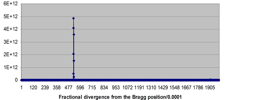
Figure 2. Intensities calculated from squared QScFs by scanning values for cs in equation 6 for a supercluster order 6 of Al6Mn [12] . The diffraction calculated is for reflections from the (2/τ, 0, 0) plane. The number of sites calculated is ~7.108. The simulated value for cs is 0.947 which is 5.3% less than expected from the corresponding angle of Bragg order 2. (courtesy Nova Science Publishers).
the ordinate scale in Figure 2. A second limiting cause for resolution is experimental, due to beam divergence, lens aberrations, thermal diffuse scattering, field aperture, specimen thickness etc., all typical features in diffraction data. A third and significant source of broadening is quasicrystal defects. All crystals contain defects, but their spatial frequency in metastable quasicrystals should be presumed comparatively high. Structural vacancies and icosahedral holes should be expected to induce finite coherence and distinct supercluster boundaries. There is evidence for some of these; but not yet for all, since they have not been properly examined with an adequate diffraction theory.
With double precision arithmetic, equation 2 operating on a supercluster order 3 gives the equivalent result to Equation (6). The latter method provides calculations at higher order and precision. The process is neither too complicated not too simple. Quasi structure factors, calculated by quasi-scattering-factors, have appropriate complexity. These geometric computations demonstrate a potential for generic applications in physics, including measurement of periodic structures by geometric probes with new functionality.
3.2. Defects
We assume that the structure is driven by the extremely high atomic density of the unit cell with pentagonal close packed planes, two on each of six normals. The cluster is not quite so dense. At its center twelve icosahedral sites are occupied by only four atoms [12] ; the other sites being too closely spaced to fit an Al atom. This has unit length in icosahedral coordinates. The center therefore contains eight vacancies, each within close range of neighboring filled sites. The sites lie on an icosahedron with edge width 1/τ. The vacancies are mobile and are consistent with effects observed in mechanical and other properties etc [21] [22] . The supercluster contains a hole on an icosahedron with edge width τ. The space is badly proportioned to fit unit cells, but there are various ways in which interstitials may occupy it. There is an outstanding need for dark field electron microscope imaging, to fill the data gap. In higher order superclusters, the interstitials may be made partly from unit cells. Defects due to both central holes and to supercluster boundaries may be expected to reduce the peak width resolution that is measured in diffracted beams. Owing to the lack of data and the variety of possibilities, systematic calculations on hole and boundary effects are ignored in the quasi structure factor calculations. It is likely that details of specimen preparation will affect measured resolution.
However, the more common vacancies due to paired sites at close range in a cluster hole are accounted probabilistically. Each Al atom in the ideal structure is either an edge-sharing site (counted in two neighboring cells, or sometimes on three neighboring atoms at a triple point where three neighbouring cells meet) or it is a vacant site. The latter is paired with a close neighbor on the neighboring cell. These atoms are all probabilistically counted with atomic scattering factors of fAl/2 for all Al atoms not located on triple points. Then fAL/3 is used instead, and counted separately in three different unit cells. Thus each Al atom in the ideal structure is accounted once.
Among the many calculations we have performed on both ideal logarithmically periodic structures of various sizes or in significant but imaginary configurations [23] ; and on models drawn from experimental micrographs [24] , consistent conclusions can be drawn with respect to resolution. Quasi structure factors show systematic narrowing with increasing sample size, reaching to the sharp diffraction line in a supercluster order 6 with ~108 atomic sites (Figure 2). This set of simulations is generally consistent with the line width being due to statistics involved in overlap between populations on atomic planes with the periodic wave of the probe. As illustrated in Figure 1, the various slopes on the Bloch wave functions that scatter on atoms achieve greater selectivity with increasing sampling.
The most important point to be made in this context is as follows: whether the quasicrystal is a defective logarithmically periodic solid or whether this is an ideal representation of quasicrystals, are two considerations that are less significant than the simple fact that they give us new physics.
3.3. Understanding the Metric
For reasons already described, the aperiodic structure that is evident in electron micrographs cannot scatter X-rays or electron beams according to Bragg’s law. The simulations of scattering due to ideal hierarchic structures show that the diffraction is not only sharp, but also consistent with intensities and symmetry found in experimental diffraction patterns. The simulation employs a metric, cs , that is measured by scanning to find the maximum simulated intensity for the diffraction. The maxima also determine secondary features, such as second order n = 2 scattering, which has a simple explanation, namely the approximately half integral locations of atoms at short range.
Can an equally simple explanation be given for the value of the metric? The short answer is, “Sort of”. Science should be made a simple as possible but not simpler. The value of the compromise spacing effect cs is found by simulation. Approximate values that correspond to the simulated value have been suggested for example π/2τ or 2.5/τ2, but reasoning is at best plausible. Two brute facts are: firstly there must be a metric because of the ordering implicit in the diffraction pattern from the aperiodic structure; and secondly this metric is found by simulation on the hierarchic model. The simplest explanation is the maximum overlap illustrated in Figure 1 and elsewhere [12] .
3.4. Quasi Bloch Waves
Figure 1 contained, in illustration, a Bloch wave that results from a periodic incident beam that interacts with a geometric lattice. In the light of the geometric diffraction pattern, it is useful to compare this trigonometric Bloch wave with what may be considered as a quasi Bloch wave having a geometric profile. The Bloch wave construction is an important feature in electron microscopy and is an essential feature in high resolution transmission electron microscopy. Any reliable interpretation will use it in simulations of through focal series. In particular, the construction is used to understand pendellösung contrast in fringes used to measure the thickness of thin metallic foils [19] . For thin crystals oriented to the two beam Bragg conditions, two components are considered in the Bloch wave. One is a cosine wave originating on the diffracting atomic planes; the other a sine wave with the same origin. The two waves are subject to different crystal potentials and propagate with different wave lengths and extinction distances, ξ1, ξ2. The difference causes the thickness fringes at the edges of a small hole in an electro-polished foil. The amplitudes of the two components mutually oscillate. In the matrix fcc phase of AlxMn melt spun alloy, the thickness fringes were more evident than in the neighboring quasicrystalline phase [25] [26] .
The geometric diffraction pattern implies on the one hand a geometric energy band structure [1] for low energy nearly free electrons, and at the same time for high energy electrons, used for illumination in the transmission electron microscope, corresponding geometric dispersion [2] . Equation (3) shows that the Bloch wave that can be expressed on a trigonometric basis may also be expressed on a geometric basis. In the two beam condition, the Bloch wave is expressed in its two components, φB = φ1 + φ2. The coupled waves interfere and interact as the Bloch wave passes down the quasicrystal. Meanwhile the two beam condition selected by apertures in the back focal plane of an imaging lens cause many terms in equation 3 to interfere destructively. By assuming orthogonality between them when integrated over long distances, the following delta function will make the same selection.
 (7)
(7)
Then, in the normal way of coupling [19] , making φ1 the zero order beam incident at the quasi Bragg angle off the vertical, represented by z coordinates:

and
 (8)
(8)
This application illustrates the physical justification for the assumption of orthogonality between the geometric terms: They are eigenfunctions expressed in diffraction.
4. Conclusion
The translational symmetry in crystals, which provides sharp diffraction on a reciprocal lattice, is replaced in hierarchic structures by logarithmically periodic quasi-scattering-factors. These produce sharp diffraction in geometric space. The clusters and superclusters are intermediate structures of equal complexity that iterate with constantly stretching order and size. They mediate the scattering due to unit cells throughout the whole, rank 3, quasicrystal. Excepting the tentatively explored role of defects, the scattering atoms lie generally on hierarchic nodes that scatter periodic waves onto a precise geometric quasi-lattice. Line widths depend on the statistics of overlap among the aperiodic, planar, atomic populations with the periodic probe.
Cite this paper
Antony J.Bourdillon, (2016) Hierarchic Computations in Geometric Space—Showing Sharp Diffraction in Quasicrystals. Journal of Modern Physics,07,43-50. doi: 10.4236/jmp.2016.71005
References
- 1. Bourdillon, A.J. (2009) Solid State Communications, 149, 1221-1225.
http://dx.doi.org/10.1016/j.ssc.2009.04.032 - 2. Bourdillon, A.J. (2010) Quasicrystals’ 2D Tiles in 3D Superclusters. UHRL, San Jose, pp. 48-52.
- 3. Bourdillon, A.J. (2010) Quasicrystals’ 2D Tiles in 3D Superclusters. UHRL, San Jose, ch. 2.
- 4. Bourdillon, A.J. (2009) Quasicrystals and Quasi Drivers. UHRL, San Jose.
- 5. Bourdillon, A.J. (2014) Journal of Modern Physics, 5, 488-496.
http://dx.doi.org/10.4236/jmp.2014.56060 - 6. Bourdillon, A.J. (2015) Log-Lin Metric in Quasicrystals. Youtube.
http://www.youtube.com/watch?v=fH2vI_WX-wQ - 7. Steurer, W. (2004) Z. Kristallogr, 219, 391-446.
- 8. Bourdillon, A.J. (2012) Metric, Myth and Quasicrystals. UHRL, San Jose, p. 82.
- 9. Bourdillon, A.J. (2014) Journal of Modern Physics, 5, 1079-1084.
http://dx.doi.org/10.4236/jmp.2014.512109 - 10. Bourdillon, A.J. (2012) Metric, Myth and Quasicrystals. UHRL, San Jose, p. 40.
- 11. Bourdillon, A.J. (2010) Quasicrystals’ 2D Tiles in 3D Superclusters. UHRL, San Jose, pp. 62-72.
- 12. Bourdillon, A.J. (2011) Logarithmically Periodic Solids. Nova Science, New York, p. 42.
- 13. Bourdillon, A.J. (2013) Micron, 51, 21-25.
http://dx.doi.org/10.1016/j.micron.2013.06.004 - 14. Bourdillon, A.J. (2009) Quasicrystals and Quasi Drivers. UHRL, San Jose, p. 100.
- 15. Shechtman, D., Blech, I., Gratias, D. and Cahn, J.W. (1984) Physical Review Letters, 53, 1951-1953.
http://dx.doi.org/10.1103/PhysRevLett.53.1951 - 16. Bursill, L.A. and Peng, J.L. (1985) Nature, 316, 50-51.
http://dx.doi.org/10.1038/316050a0 - 17. Bourdillon, A.J. (2012) Metric, Myth and Quasicrystals. UHRL, San Jose, 29, pp. 45-50.
- 18. Cullity, B.D. (1978) Elements of X-Ray Diffraction. Addison-Wesley, Addison.
- 19. Hirsch, P., Howie, A., Nicholson, R.B., Pashley, D.W. and Whelan, M.J. (1977) Electron Microscopy of Thin Crystals. Krieger, New York.
- 20. Huntley, H.E. (1970) The Divine Proportion. Dover, New York.
- 21. Bourdillon, A.J. (2011) Logarithmically Periodic Solids. Nova Science, New York, p. 48.
- 22. Puckerman, B.E., Ed. (2011) Quasicrystals, Types, Systems and Techniques. Nova Science, New York.
- 23. Bourdillon, A.J. (2012) Metric, Myth and Quasicrystals. UHRL, San Jose, pp. 40-42.
- 24. Bourdillon, A.J. (2010) Quasicrystals’ 2D Tiles in 3D Superclusters. UHRL, San Jose, pp. 68-72.
- 25. Bourdillon, A.J., Tebby, G.P., Warner, T.J. and Stobbs, W.M. (1987) Philosophical Magazine Letters, 55, 115-122.
- 26. Bourdillon, A.J. (1987) Philosophical Magazine Letters, 55, 21-26.
NOTES

1Two notions are common in quasicrystallography. Firstly confusion: the diffraction is so weakly understood that it is called by the self-contradiction of Bragg diffraction in Fibonacci sequence, with a metric that is chosen, not measured; secondly abstraction: for lack of understanding, Bragg’s law is applied to individual diffracted beams, supposedly due to respective interplanar spacings, while ignoring the variety of other spacings that are supposed to scatter incoherently. In fact the crystallographic and comprehensive notion given in this paper considers all scattering, found to be coherent in geometric space.

2In icosahedral units, the lattice parameter a = 1. The conversion to SI units is given in ref. [4] .