Journal of Modern Physics
Vol.4 No.6(2013), Article ID:32950,8 pages DOI:10.4236/jmp.2013.46101
Transverse Stability in the Discrete Inductance-Capacitance Electrical Network
1Laboratory of Mechanics, Department of Physics, Faculty of Sciences, University of Yaounde I, Yaounde, Cameroon
2Nonlinear Physics and Complex Systems Group, Department of Physics, The Higher Teachers’ Training College, University of Yaounde I, Yaounde, Cameroon
Email: *tebue2007@gmail.com
Copyright © 2013 Eric Tala-Tebue, Aurelien Kenfack-Jiotsa. This is an open access article distributed under the Creative Commons Attribution License, which permits unrestricted use, distribution, and reproduction in any medium, provided the original work is properly cited.
Received March 2, 2013; revised April 3, 2013; accepted April 30, 2013
Keywords: Two-Dimensional Nonlinear Schrödinger Equation; Exact Transverse Solution; Stability; Modulational Instability
ABSTRACT
This work investigates the dynamics of modulated waves in a coupled nonlinear LC transmission line. By means of a method based on the semi-discrete limit and in suitably scaled coordinates, we derive the two-dimensional NLS equation governing the propagation of slowly modulated waves in the network. The exact transverse solution is found and the analytical criteria of stability of this solution are derived. The condition for which the network can exhibit modulational instability is also determined. The exactness of this analytical analysis is confirmed by numerical simulations performed on the exact equation of the network.
1. Introduction
Nonlinear dissipative waves have attracted considerable attention in recent years as a result of their multiple applications in many systems. These applications can be observed in different fields of the research. Among these domains, we can list biology, chemistry and physics to mention a few. In physics precisely, nonlinear electrical transmission lines (NETLs) are good examples to provide a useful way to check how the nonlinear excitations behave inside the nonlinear medium. In particular, one of their importance lies on the easy and rapid technique to investigate the behavior of nonlinear excitations throughout the waveguide. Moreover, it allows investigations of new erotic designs. Following these introductive studies longtime after, a great number of works have been done on NETLs. Thus, the first nonlinear and dissipative transmission line was built by Hirota and Suzuki [1]. Several investigations have been done to improve this first line due to the fact that electrical transmission lines are very convenient tools to study the fascinating properties of nonlinear waves [2,3]. Distributed electrical transmission lines that consist of a large number of identical sections have been used for the experimental study of the propagation of Korteweg-de Vries (KdV) solitons which satisfy the famous KdV equation. It has been shown that the equation governing the physics of nonlinear electrical line can be reduced to a cubic nonlinear Schrödinger equation or a pair of coupled nonlinear Schrödinger equations, the complex Ginzburg-Landau equation or the coupled complex Ginzburg-Landau equations [4-6]. Recently, many works were done on NETLs by Tala and coworkers and by Togueu et al. [4,7]. The first authors show how to solve the crucial problem of mixing waves in coupled nonlinear LC transmission lines by using only half of the total number of additive linear inductors compared to that found in the literature; they also exploit the features of the modulational instability (MI) of each of two modes through the network. The second authors study the supratransmission phenomenon in a discrete electrical lattice with nonlinear dispersion; they introduce the driven Salerno equation describing the dynamics of modulated waves in a discrete nonlinear electrical transmission lattice submitted to a periodic driving source with constant amplitude and show that the driving amplitude must be slightly above the threshold to achieve a good supratransmission.
MI leads to a self-induced modulation of an input plane wave with the subsequent generation of localized pulses; it is responsible for many interesting physical effects such as the formation of envelope solitons [8]. A soliton can be viewed as the result of an instability that leads to a self-induced modulation of the steady state produced by the interaction between nonlinear and dispersive effects. Marquié et al. [8,9] presented a careful and quantitative experimental analysis of modulational instability and the generation of either envelope or hole solitons, depending on an appropriate choice of the carrier wave frequency. The field of solitons in general and the field of Telecommunications solitons in particular have grown enormously since the word soliton was coined. Most of this growth occurred over the last 10 years or so, during which many new kinds of Telecommunications solitons were identified.
The purpose of this work is to conduct the linear stability analysis of solitary waves propagating in coupled nonlinear LC transmission lines with respect to longwavelength transverse perturbations on the basis of the nonlinear Schrödinger (NLS) equation. Therefore, our investigation of the transverse perturbations to the twodimensional NLS equation of the NETLs may be helpful in other fields of physics. The paper is organized as follows: in Section 2, we present the basic characteristics of the coupled NETL under consideration; in the semi-discrete limit, we derive the amplitude equations and the two-dimensional NLS equation governing the propagation of slowly modulated waves in the network. The solution of NLS, the stability and the condition for which our network can support the pulse solution are determined in Section 3. In Section 4, numerical experiments are done in order to verify the validity of the theoretical predictions. Finally, concluding remarks are presented in Section 5.
2. Main Characteristics of the Coupled NETLs and Dynamic Equation
The standard nonlinear discrete LC line is a structure made of elementary cells which consist of an inductance L and a nonlinear capacitor C(V) [10]. Many schematic electrical lattices have already been considered in the literature [4]. The model used in this work consists of a nonlinear network with many coupled nonlinear LC dispersive transmission lines. We imagine that there are many identical dispersive lines which are coupled by means of inductance L3 at each node, as shown in Figure 1. Each section of line consists of a constant inductor L1 in the series branch and a nonlinear capacitor of capacitance C(Vn,m) in parallel with a constant inductor L2 in the shunt branch. The nodes in the system are labeled with two discrete coordinates n and m, where n specifies the nodes in the direction of propagation of the pulse, and m labels the lines in the transverse direction.

Figure 1. Schematic representation of the NETL.
In the network, nonlinearity is introduced by a varicap diode which admits that the capacitance varies with the applied voltage. The voltage dependence relation is assumed to have a polynomial form given by
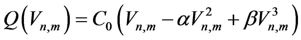 (1)
(1)
where  are constants. In the present work, we set
 . Applying Kirchoff’s laws to this system leads to the following set of propagation equations:
 (2)
(2)
with .
.
Equation (2) is the differential equation governing the wave propagation in the network under consideration. As one can see, all of the lines have the same characteristic frequency. This is due to the fact that all of the lines are identical.  is the coupling frequency. The properties of the network can be studied by using a solution of the form
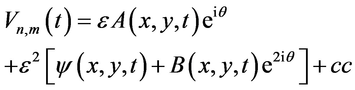 (3)
(3)
where  is the phase and “cc” stands for the complex conjugated of the preceding expression; k and q are the wave numbers respectively in the n and m direction;
  is the angular frequency;
  is a small parameter. For the semi-discrete approximation, we set
 (4)
(4)
to obtain the short wavelength envelope solitons; vg and ug are the group velocities respectively in the n and m direction. Substituting Equation (3) into Equation (2), we obtain different equations as power series of .
.
1) The coefficient of , proportional to exp(iθ), gives the dispersion relation
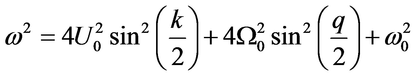 (5)
(5)
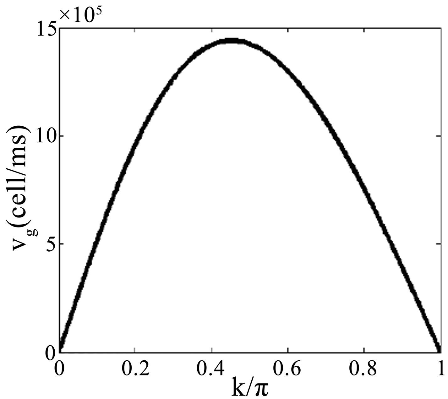
This dispersion relation shows that our network is a band-pass filter. Figure 2 represents the evolution of the angular frequency in the first Brillouin zone for the n direction. To plot Equation (5), we fix . The group velocity is taken to be
 (6)
(6)
This group velocity is represented in Figure 3.
2) The coefficient of , proportional to exp(2iθ) leads to the following relation:
 (7)
(7)
3) From the coefficient of , proportional to exp(iθ),
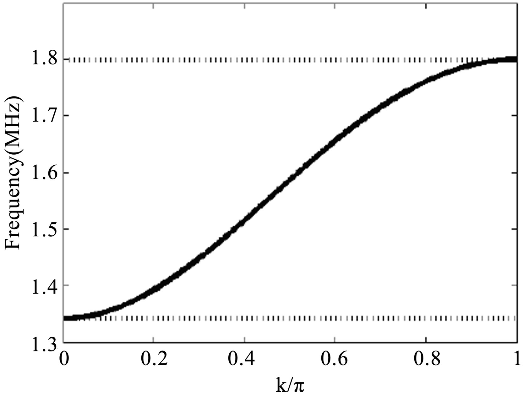
Figure 2. Dispersion graph obtained with L1 = L2 = L3 = 0.22 mH; C0 = 320 pF.
we obtain the following two-dimensional nonlinear Schrödinger equation for A:
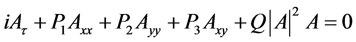 (8)
(8)
with the following definitions
 (9)
(9)
The numbers P1, P2 and P3 are the dispersion coefficients, while Q is the nonlinearity coefficient of the nonlinear Schrödinger equation.
3. Solution and Stability of NLS
The focal point here corresponds to the determination of the solution of Equation (8). Before the discovery of solitons, mathematicians thought that nonlinear differential equations could not be solved, at least not exactly. However, solitons lead to the recognition that through a combination of such diverse subjects as quantum physics and algebraic geometry, one can actually solve some nonlinear equations exactly. This innovation opens up a wide window in the world of nonlinearity [11]. With the development of soliton theory, many powerful methods for obtaining the exact solutions of NETLs have been presented [12-16]. In the present case, we use the variational method [17]. This method is a powerful solution method for the computation of exact traveling wave solutions. Because of the complexity of the nonlinear wave equations, there is no unified method to find all solutions of these equations. Here, we look for a propagating wave under the form:
 (10)
(10)
where a(z) is the amplitude, g(z) is the phase,  represents the spectral parameter of the wave and
 the single variable for the amplitude, depending on ve which is the velocity of the wave packet. By substituting Equation (10) into the two-dimensional NLS Equation (8), and equating real and imaginary parts to zero, the following two coupled ordinary differential equations are obtained:
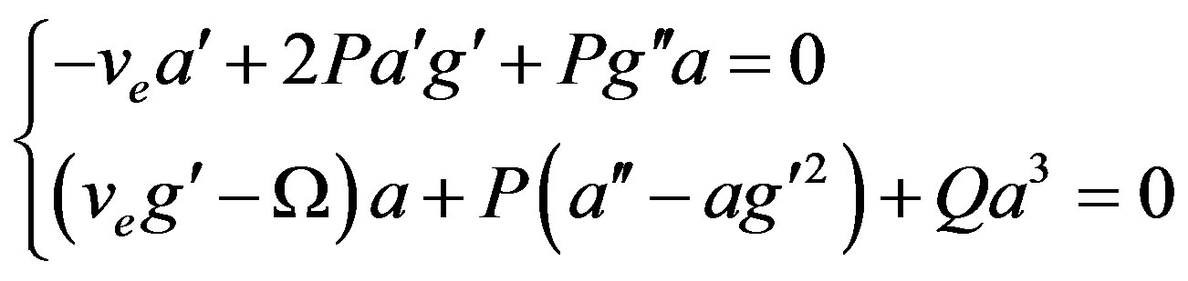 (11)
(11)
where the prime stands for derivation with respect to z and . By multiplying the first equation of (11) by a(z) and integrating once, it follows that the phase g is related to the amplitude a(z) through the expression:
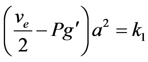 (12)
(12)
where k1 is the constant of integration, which can naturally be taken as k1 = 0 for all continue solution at the origin a = 0. Taken then k1 = 0, Equation (12) yields
 (13)
(13)
By substituting Equation (13) into the second equation of (11), we arrive to the following differential equation satisfied by the amplitude a(z):
 (14)
(14)
from which the first integral is obtained by multiplying Equation (14) by  and integrating the resulting equation:
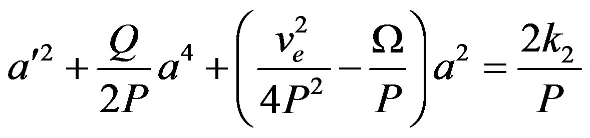 (15)
(15)
with k2, another constant of integration. Let us mention that, Equation (15) can be also derived from the auxiliary Hamiltonian  and lagrangian
  defined as follows:
 (16)
(16)
This Hamiltonian may be viewed as the energy of a particle with an effective mass m(a) = 1 moving in the effective potential
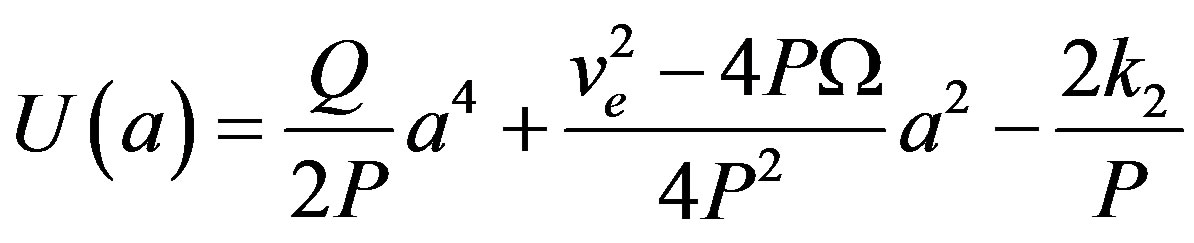 (17)
(17)
It is obvious that Equation (14) can be transformed into the following equivalent autonomous dynamic system:
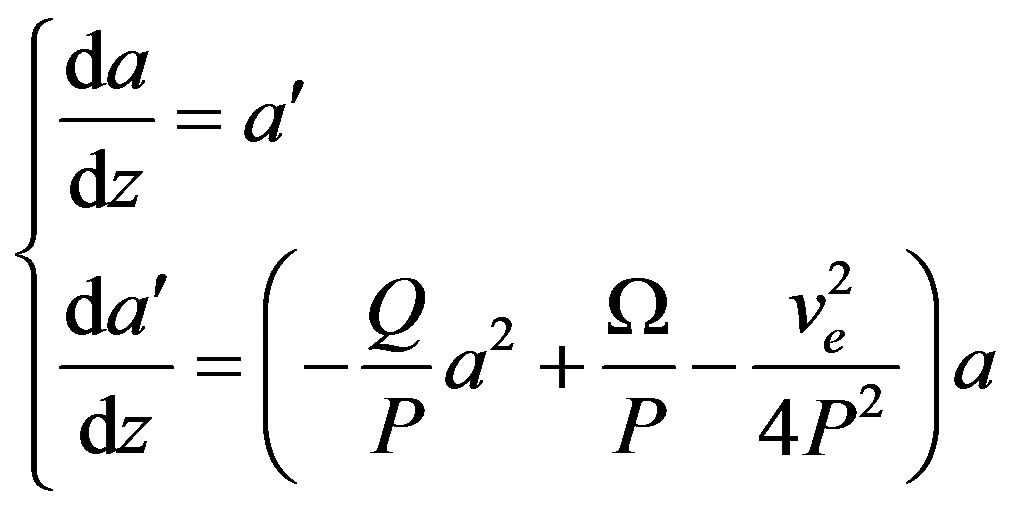 (18)
(18)
where solutions are the fixed points of the system. The number of equilibrium points, and consequently the dynamic of this system depend on the sign of the quantity
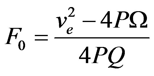 (19)
(19)
In fact, when F0 > 0, the system (18) admits only the equilibrium point (0, 0) and consequently, no nonlinear localized wave (NLW) can be obtained. However, for F0 < 0, the system admits three equilibrium points: (0, 0) and (0, ±Aeq), with
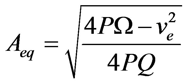 (20)
(20)
From the linear stability analysis, it appears that the stability of these equilibrium points depends on the sign of the product PQ (the saddle point is obtained if
 and the center point else). In factwhen PQ > 0, the equilibrium point (0, 0) is a saddle while the two others, (0, ±Aeq), are the centers. This analysis is confirmed by the phase plane plot of the system sketched in Figure 4. (1) obtained for the numerical values of parameters: P = Q = 1.0, ve = 0.0 and Ω = 1.0; that is PQ > 0 and
 , in which closed trajectories are presented. These trajectories indicate that small oscillations of the system as well as periodic solutions are possible and are separated by the homoclinic orbit known as the separatrix characterizing the existence of pulse soliton or bright solitary waves (BSW) in the context of the NLS system. These BSW are nonlinear solutions of Equation (18) with the vanishing boundary conditions
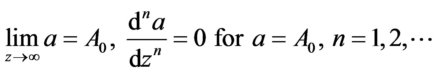
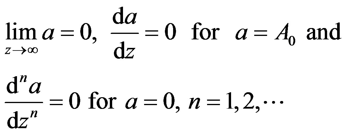 (21)
(21)
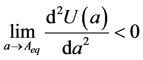
where A0 is the maximum amplitude of the envelope wave. The condition (21) leads to the following constraint to be satisfied by the integrating constant k2 and the spectral parameter Ω
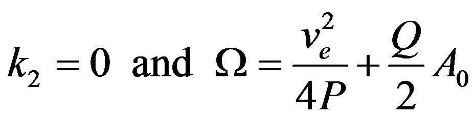 (22)
(22)
However, when PQ < 0, there is a change in the properties of the above equilibrium points; (0, 0) becomes a center while (0, ±Aeq) are the saddle points. The phase plane plot sketched in Figure 4. (2), obtained for P = −Q = 1.0, ve = 0.0 and Ω = −1.0; that is PQ < 0 and  show a changes in the behavior of the system. The closed and open orbits are now separated by the heteroclinic orbits which evidence the existence of dark solitary waves (DSW) which satisfying the non vanishing boundary conditions
 (23)
(23)
from which the following expressions of the spectral parameter and the integration constant are obtained:
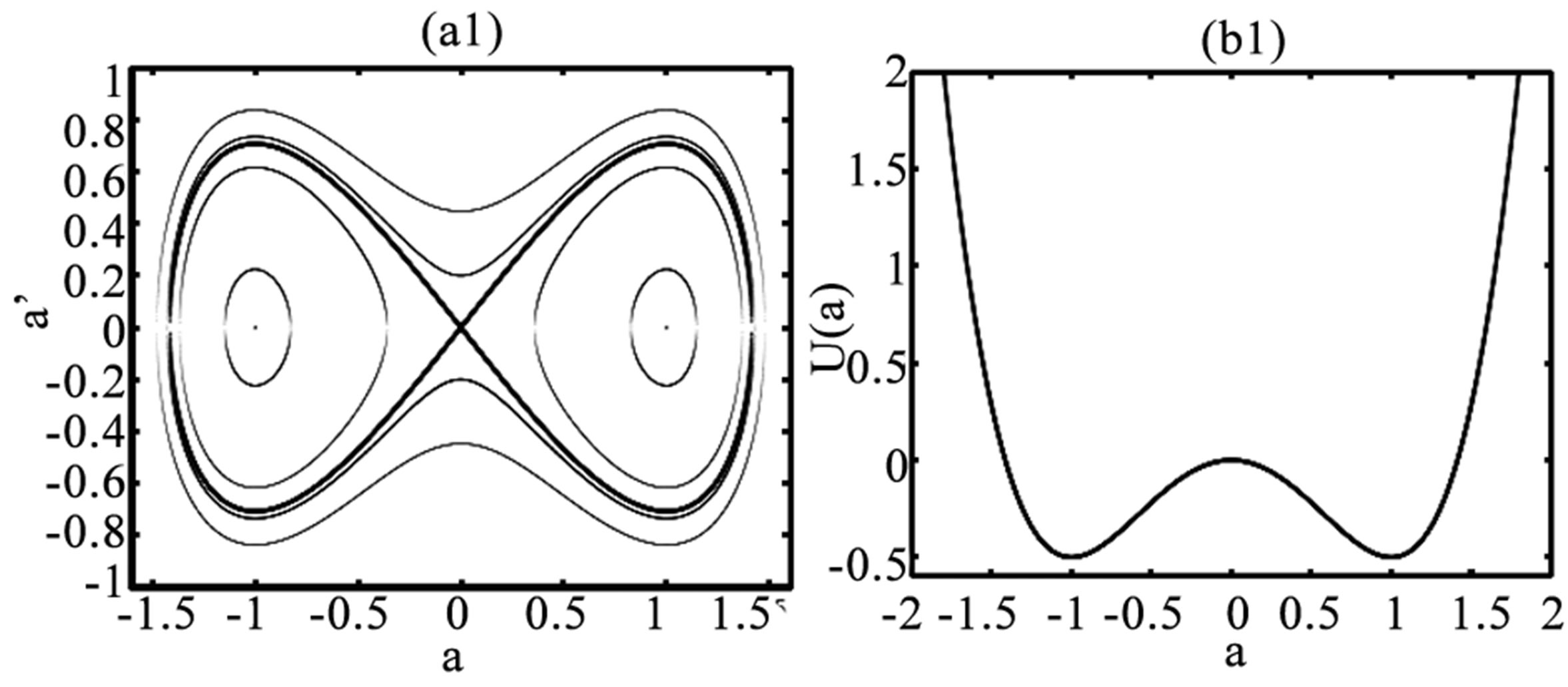

Figure 4. Phase plane plot (a), and the effective potential U(a) (b) of the system described by the NLS equation. The homoclinic orbit (a1) and the heteroclinic orbit (a2) are plotted in bolt lines.
 (24)
(24)
The plot of the effective potential U(a) indicates the presence of a double wells when PQ > 0 and a single well for PQ < 0 which are in agreement with results of the phase plane plots.
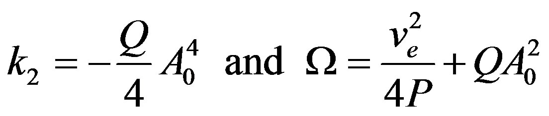
Now we focus our attention on the derivation of bright solution of the NLS. For this end, the integration constant k1 = 0, while k2 and the spectral parameter Ω will be taking as given in Equation (22); thus, Equation (15) can be rearranged as
 (25)
(25)
with ;
;  is a parameter describing the pulse width. From Equation (13), the phase g(z) is given by
 (26)
(26)
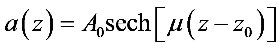
where z0 is the initial position of the wave which can be equal to zero. Hence the solution of the NLS equation can explicitly be rewritten as:
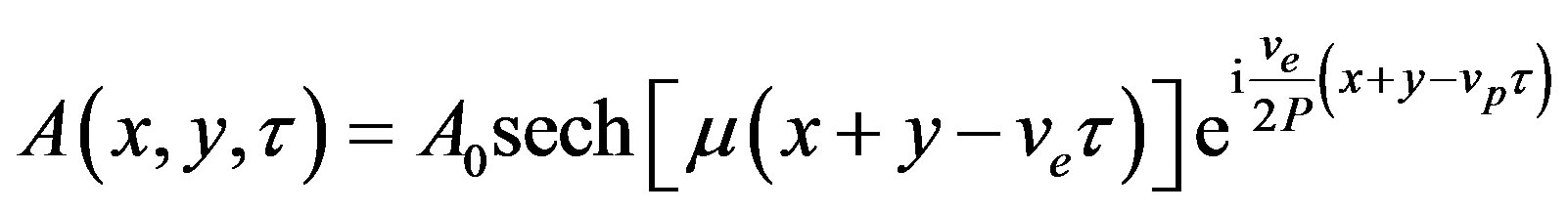 (27)
(27)
vp is the carrier velocity, with the following expression
 (28)
(28)
As for the particular case of solution with stationary phase in time (vp = 0), we have:
 (29)
(29)
Having found this solution, we then check its stability. The stability of the BSW is determined here by the dependence of the norm (the power) on the velocity ve. Solitons are stable if dN/dve > 0 and unstable otherwise [18]. For the model considered here, N(ve) can be found analytically as , leading to:
 (30)
(30)
Substituting the ve obtained in Equation (29) into (30), one obtains
 (31)
(31)
which is an increasing function of the envelope velocity for PQ > 0 and then pulse soliton is stable.
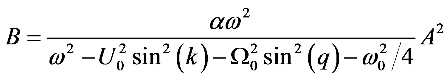
To determine the conditions of instability of the modulated waves in the network, we use the plane wave solution given below:
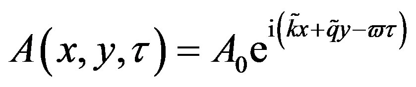 (32)
(32)
By inserting Equation (32) into Equation (8), we have the following dispersion relation:
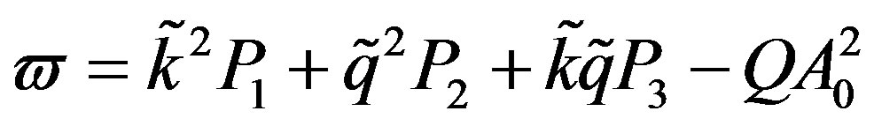 (33)
(33)
The linear stability of this continuous wave can be investigated by looking for a solution of the form
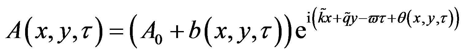 (34)
(34)
where  and
and  are small perturbations for the amplitude and for the phase respectively; they can be writen as follow:
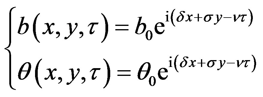 (35)
(35)
Substituting (34) and (35) into Equation (8), one obtains a system for the perturbations. For the nontrivial solutions of this system, we then have:
 (36)
(36)
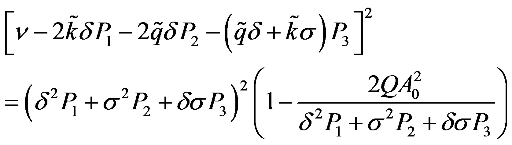
It appears that the behavior of  depends on the quantity
 . On one hand, if this quantity is negative, the plane wave solution of NLS equation is stable. On the other hand, if this quantity is positive,
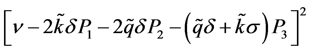 could be negative under certain conditions and the consequence is that the plane wave solution of NLS equation is unstable; hence, it appears MI phenomenon in the line. This instability induces the formation of small wave packets or envelope pulse solitons train, solution of the NLS equation (8).
4. Numerical Experiments
We present in this section the numerical experiments on the propagation of slowly modulated waves in the network, this to check the analytical calculations presented in the previous sections. The numerical experiments are carried out in Equation (2) describing the propagation of waves in the NETL of Figure 1. The wave is introduced in the following form
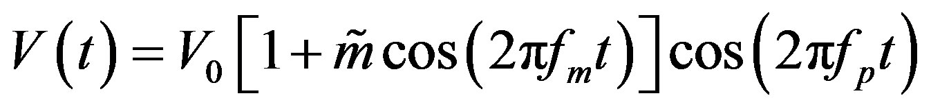 (37)
(37)
where fm is the modulation frequency, V0 is the amplitude of the wave and  is the modulation rate. We take fm = 54 kHz, V0 = 0.2 V and
 . A fourth-order RungeKutta algorithm has been used and a normalized integration time step
  is used for numerical simulations. Similarly, the number of cells N in the n direction is chosen to be equal to 3000 and we have used periodic boundary conditions so that we do not encounter the wave reflection at the end of the line. In the m direction, we have taken M = 18. The parameters of the network are the same as in Figure 2. This simulation is made in the case where
 ,
,  that is
 . We take the carrier frequency fp = 1752 kHz.
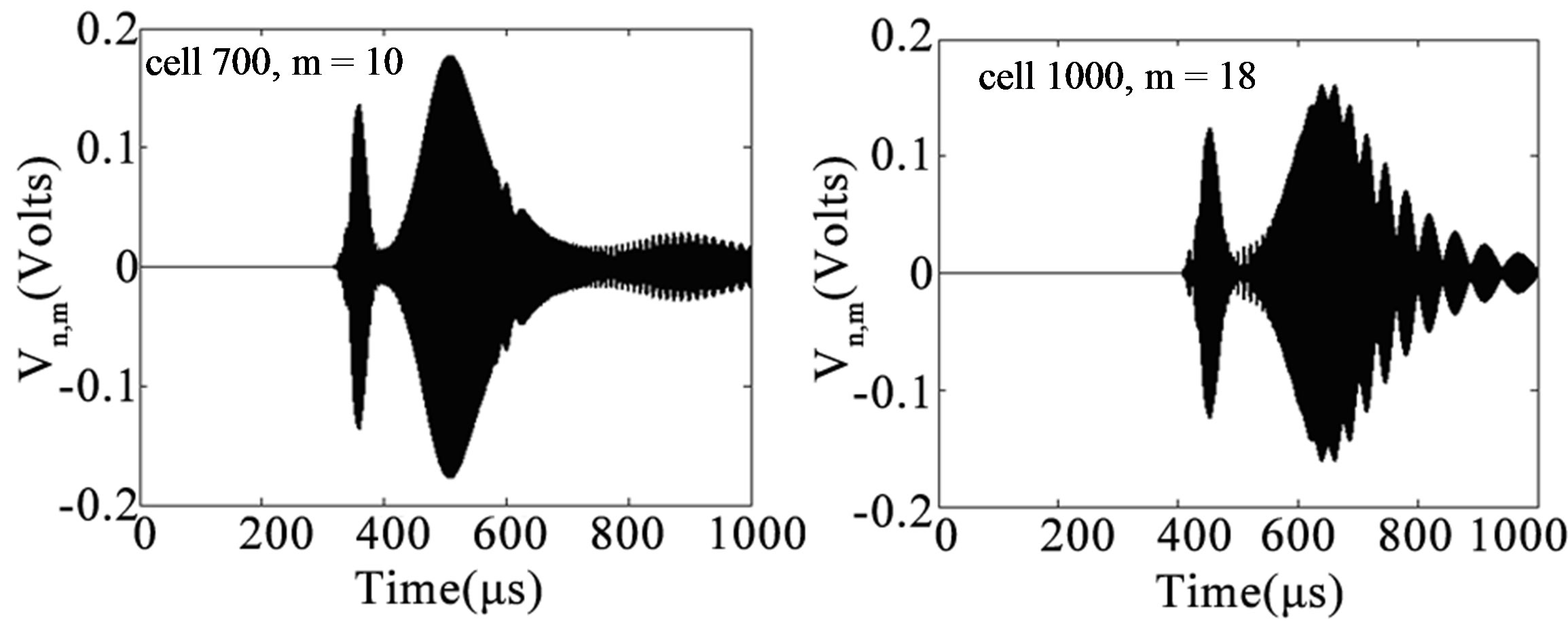
Figure 5 shows the evolution of the plane wave in the network. On this figure, we observe examples of the MI exhibited by the network. As time goes on, the wave exhibits a modulation of its amplitude, which leads to the formation of wave packets which is in agreement with the analytical calculations. In the view to consolidate the validity of preceding results, we propagate the solution of the NLS since the above observed Benjamin-Feir instability constitutes the proof that the network can support envelope solitons. For this purpose, we take as input voltage the profile of a modulated soliton given by
 (38)
(38)
In Figure 6, we depict the time evolution of relation (38) in the line characterized by equation (2) for the same frequency as in Figure 5. This result confirms the fact that our network can support the pulse soliton.
In this last figure the, we can observe the fission of two-bound solitons; this can be explained by the additional terms in the NLS equation. A similar phenomenon has been already obtained in the context of higher-order NLS by David Yemélé et al. [10].
5. Conclusion
In this work, we have considered a system of coupled nonlinear dispersive transmission lines and we have
 (a) (b)
Figure 5. Propagation of waves through the network at the cell 700 for m = 10 (a) and at the cell 1000 for m = 18 (b).

Figure 6. Propagation of envelope soliton signal voltage as a function of cell number n at different times. The left column is obtained for t1 = 450 μs while the right is obtained for t2 = 850 μs. The parameters are the same as in Figure 5.
shown that the voltage for the transmission lines is described by a two-dimensional nonlinear Schrödinger equation. The exact transverse solution has been found and its stability has been studied. The condition for which the network can exhibit modulational instability is also determined and we observe a good agreement between analytical calculations and numerical simulations.
6. Acknowledgements
Eric Tala-Tebue acknowledges help made by Agostiny Marrios Lontsi for the payment. The authors are grateful to the Journal of Modern Physics for financial support in publication.
REFERENCES
- R. Hirota and K. Suzuki, Journal of the Physical Society of Japan, Vol. 28, 1970, pp. 1366-1367. doi:10.1143/JPSJ.28.1366
- A. C. Scott, “Active and Nonlinear Wave Propagation in Electronics,” Wiley, New York, 1970.
- M. Remoissenet, “Waves Called Solitons,” 2nd Edition, Springer, Berlin, 1996. doi:10.1007/978-3-662-03321-0
- E. Tala-Tebue, A. Kenfack-Jiotsa, M. Hervé TatchouNtemfack and T. C. Kofané, Communication in Theorical Physics, 2013, in Press.
- S. Abdoulkary, T. Beda, S. Y. Doka, F. II Ndzana, L. Kavitha and A. Mohamadou, Journal of Modern Physics, Vol. 3, 2012, pp. 438-446 doi:10.4236/jmp.2012.36060
- A. Kenfack-Jiotsa and E. Tala-Tebue, Journal of the Physical Society of Japan, Vol. 80, 2011, Article ID: 034 003 doi:10.1143/JPSJ.80.034003
- A. B. T. Motcheyo, C. Tchawoua, M. S. Siewe and J. D. T. Tchameu, Communications in Nonlinear Science and Numerical Simulation, Vol. 18, 2013, pp. 946-952. doi:10.1016/j.cnsns.2012.09.005
- P. Marquie, J. M. Bilbault and M. Remoissnet, Physical Review E, Vol. 49, 1994, pp. 828-835. doi:10.1103/PhysRevE.49.828
- P. Marquie, J. M. Bilbault and M. Remoissnet, Physical Review E, Vol. 51, 1995, pp. 6127-6133. doi:10.1103/PhysRevE.51.6127
- D. Y. P. Marquié and J. M. Bilbault, Physical Review E, Vol. 68, 2003, Article ID: 016605. doi:10.1103/PhysRevE.68.016605
- M. Antonova and A. Biswas, Communications in Nonlinear Science and Numerical Simulation, Vol. 14, 2009, pp. 734-748. doi:10.1016/j.cnsns.2007.12.004
- S. A. El-Wakil and M. A. Abdou, Chaos, Solitons and Fractals, Vol. 31, 2007, pp. 840-852. doi:10.1016/j.chaos.2005.10.032
- W. Malfliet and W. Hereman, Physica Scripta, Vol. 54, 1996, pp. 563-568. doi:10.1088/0031-8949/54/6/003
- M. Y. Moghaddam, A. Asgari and H. Yazdani, Applied Mathematics and Computation, Vol. 210, 2009, pp. 422- 435. doi:10.1016/j.amc.2009.01.002
- E. Fan and H. Zhang, Physical Letters A, Vol. 246, 1998, pp. 403-406. doi:10.1016/S0375-9601(98)00547-7
- R. Hirota, “The Direct Method in Soliton Theory,” Cambridge University Press, Cambridge, 2004. doi:10.1017/CBO9780511543043
- M. T. Darvishi and M. Naja, International Journal of Applied Mathematical Research, Vol. 1, 2012, pp. 1-7.
- W. Krolikowski and O. Bang, Physical Review E, Vol. 63, 2000, Article ID: 016610. doi:10.1103/PhysRevE.63.016610
NOTES
*Corresponding author.