ABSTRACT

We review the physics of chiral anomaly and show that the anomaly equation of 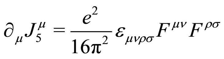is not connected to any physical observables. This is based on the fact that the reaction process of has no divergence at all, and the triangle diagrams with the vertex of describing the decay do not have any divergences either. The recent calculated branching ratio of the decay rate is found to be. Further, we discuss the anomaly equation in the Schwinger model which is known as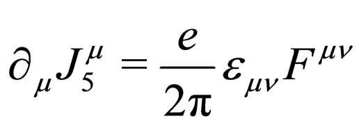, and prove that this anomaly equation disagrees with the exact value of the chiral charge in the Schwinger vacuum.Therefore, the chiral anomaly is a spurious effect induced by the regularization. In connection with the anomaly problem, we clarify the physical meaning why the self-energy of photon should not be included in the renormalization scheme. Also, we present the renormalization scheme in weak interactions without Higgs particles, and this is achieved with a new propagator of massive vector bosons, which does not give rise to any logarithmic divergences in the vertex corrections. Therefore, there is no necessity of the renormalization procedure of the vertex corrections arising from the weak vector boson propagation.

1. Introduction

The physics of the chiral anomaly in quantum field theory has been discussed quite extensively, and it is considered to be established by now [1,2]. The anomaly equation can be written as

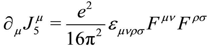(1.1)

where the axial vector current is defined as. The anomaly equation is obtained by making the regularization of the triangle diagrams which involve the vertex of [3]. This is basically because the triangle diagrams with the vertex of give rise to the apparent linear divergence and, after the regularization, one sees that the axial vector current is not conserved any more. Namely, the equation becomes just the same as (1.1). Therefore, it is stated that the axial vector current is conserved at the classical field theory, but after the regularization it is not conserved any more.

However, this is somewhat a strange statement because the triangle anomaly itself is obtained after the fields are quantized, and thus the violation of the basic conservation law like the axial vector current derived as the Noether current must have been due to an extremely special mechanism involving some physics beyond the field quantization. Therefore, we should reexamine the physical meaning of the regularization in this context. Up to now, we cannot find any convincing physics arguments of the regularization, and it should be very important to understand why the regularization scheme is considered to be “quantum”. Namely, people believe that the anomaly equation due to the regularization is a quantum effect, and therefore the axial vector current conservation law can be violated. Thus, the procedure of the regularization is considered to be somewhat beyond the field quantization. This is indeed a mystery why people believed this unphysical arguments as if they were trapped in the mass hypnosis state.

Here, we should repeatedly stress that the regularizetion is only a mathematical tool which cannot be related to a meaningful physical concept. This is in contrast to the field quantization which is directly connected to the creation and annihilation of particles. Therefore, it is clear that the regularization cannot be more fundamental than the field quantization.

There is no doubt that any physically meaningful processes are calculated without the help of the regularization as far as we make use of the renormalization scheme in a proper manner. A typical example can be indeed seen in the calculation of the anomalous magnetic moment of electron in terms of vertex corrections. In this case, the divergent terms appearing in the corresponding Feynman diagrams can be renormalized into the fermion wave function without any further procedures.

In addition to the chiral anomaly in four dimensional QED, there is an anomaly equation in the Schwinger model which is a massless QED in two dimensions. The anomaly equation for the Schwinger model can be written as

(1.2)

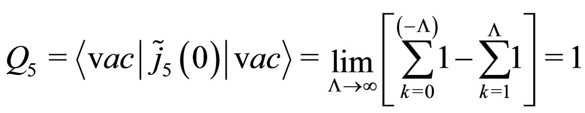
which is obtained by regularizing the vacuum charge in terms of the -function regularization method with the large gauge transformation invariance taken into account [4]. This means that Equation (1.2) represents the property of the vacuum state of the Schwinger model [5], and therefore it is not an operator equation [6]. Besides, the chiral charge can be calculated exactly without the regularization, and one sees that becomes

(1.3)

where the vacuum has two fold degeneracy, which is not resolved in the Schwinger model. On the other hand, the chiral charge predicted from Equation (1.2) depends on the vector field, and therefore the regularization induces the chiral charge which does not agree with the exact value of the chiral charge in the Schwinger model. This clearly shows that Equation (1.2) is a spurious equation which has nothing to do with real physics, even though the mathematical procedure may be correct. Here, the physics is simple, that is, the chiral charge of the Schwinger vacuum has no divergence and therefore the regularization should not be done for.

In this paper, we show that the anomaly Equation (1.1) cannot be connected to any physical processes, contrary to a naive belief. The basic reason is that the corresponding Feynman diagram of the decay has no divergence as is well known [7], and the derivative coupling of the pion-nucleon interaction can be reduced to the pseudoscalar interaction as long as one properly makes use of the axial vector current conservation law of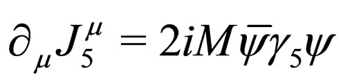. Therefore, the axial vector current interaction in connection with decay process does not produce any divergences. In addition, we show that the triangle diagrams with the axial vector current coupling which correspond to the description of the decay process have no divergences either, and the recent calculated branching ratio of the decay rate gives the predicted value of

.

Therefore there is no chiral anomaly in the axial vector current conservation law. Thus, contrary to a common belief, it is very difficult to accept that the anomaly equation can be connected to any physical observables in four dimensions.

In the last two sections, we discuss the renormalization scheme and clarify some important points in connection with physical observables. In quantum field theory, we have to rely on the perturbation theory, and therefore we should have correct information on the wave functions (or polarization vectors) of bosons. Normally we use the polarization vector to describe the wave function or spinor. However, we have never solved the equation of motion for the, and thus the determination of polarization vector from the equations of motion has been missing for free massive vector bosons as well as for free gauge fields. As one knows, the free Dirac equation is always solved by asking that the determinant of the matrix for the Dirac spinor equation should vanish(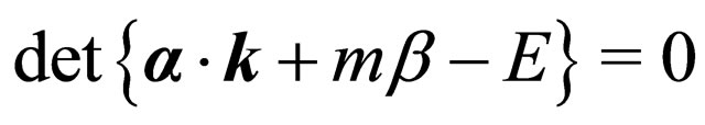), and then one can obtain the dispersion relation (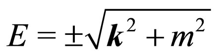), which can finally determine the wave function of the free Dirac fields. It is surprising that the same procedure has never been made for the vector bosons. Now if we carry out the same procedure for gauge fields as well as massive vector bosons, then we can obtain the correct dispersion relations, which can then determine the constraint equation for the polarization vector. We find

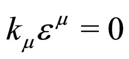(1.4)

which is just the Lorentz condition. This clearly shows that the Lorentz gauge fixing in QED is not a proper one since the condition of equation is already obtained from the equation of motion which is, of course, more fundamental than the gauge fixing. For the massive vector boson case, the situation is crucial, and it leads to a new propagator

(1.5)

Here, one can easily see that the replacement of the term by in the numerator is not allowed, and this shape of Equation (1.5) is uniquely determined. In addition, the vertex corrections of fermions due to this propagator do not have any logarithmic divergences, and this is very important and reasonable since the vertex corrections are directly related to physical observables. Therefore, we do not have to worry about the renormalization procedure in the evaluations of physical observables by the massive vector boson propagations.

2. Anomaly Equation

Here, we first discuss the anomaly problem and clarify what is the basic point of this equation in connection with physical observables. Before going to the discussion of the anomaly equation, we reconfirm that the process has no divergence, and therefore there should not be any anomalous behaviors in the theoretical evaluation of this reaction process.

2.1. No Anomaly in Process

Now, we consider the reaction process of. In this case, the interaction Lagrangian density between fermion and pion can be written as

(2.1)

where the isospin indices are suppressed. In this case, the corresponding Feynman diagrams for the reaction can be written as

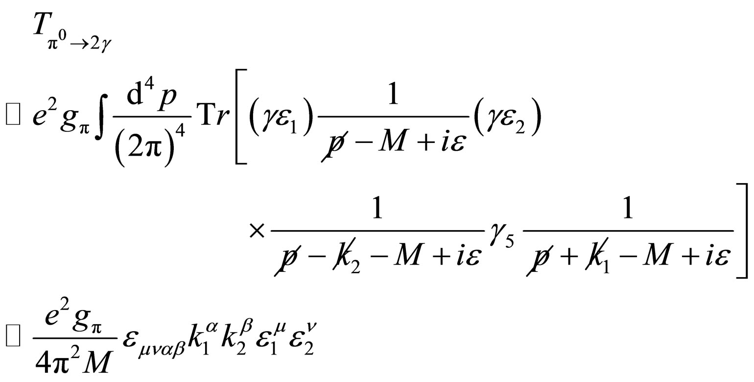(2.2)

where () and () denote the four momentum and the polarization vector of photon 1 (photon 2), respectively. Also, and satisfy the following relations of, and. Here, M and denote the nucleon and pion masses, respectively. Now, one can easily evaluate this integral and see that there is no divergence in this T-matrix calculation since the apparent linear divergence can be completely canceled out due to the Trace evaluation. In this respect, the corresponding T-matrix is finite and thus there is no chiral anomaly in this Feynman diagrams. This is, of course, well known to those physicists who make calculations by their own hand [7].

2.2. Axial Vector Coupling with Derivatives

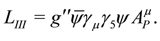
Where can we then find the anomalous behavior in the triangle diagrams? There, we have to consider the axial vector coupling in which the Lagrangian density becomes

(2.3)

In this case, if one carries out the T-matrix calculation naively, then it looks that one can find the linear divergence. Therefore, people claim that they have to regularize the T-matrix evaluation in order to obtain the finite result. In this case, they find that the axial vector current is not conserved any more, and they find the result of Equation (1.1). However, this procedure of the calculation is too naive. One has to consider the conservation of the axial vector current which can be written as

(2.4)

In this case, the axial vector coupling interaction can be rewritten as

(25)

where we have made use of the fact that the total divergence does not contribute to any physical processes, and therefore it is safely neglected. This means that the derivative coupling of the pion with the fermions can be reduced to the normal pseudoscalar interaction if one can properly make use of the axial vector current conservation law, and therefore there is no chiral anomaly even for the axial vector coupling.

2.3. Standard Procedure of Anomaly Equation

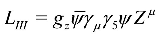
Now, we briefly review the procedure to obtain the anomaly equation which is described in field theory textbooks [1,2,8], and clarify the physics behind the equation. The starting point of the anomaly equation is the Feynman diagram which involves the triangle diagrams with three vertex interactions of, and. Here, we can write the Lagrangian density of the weak boson field and the fermion field as [9]

(2.6)

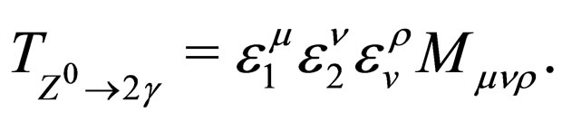
which is due to the standard electroweak interactions. In this case, the corresponding T-matrix for the boson decaying into two photons can be written as [2,8]

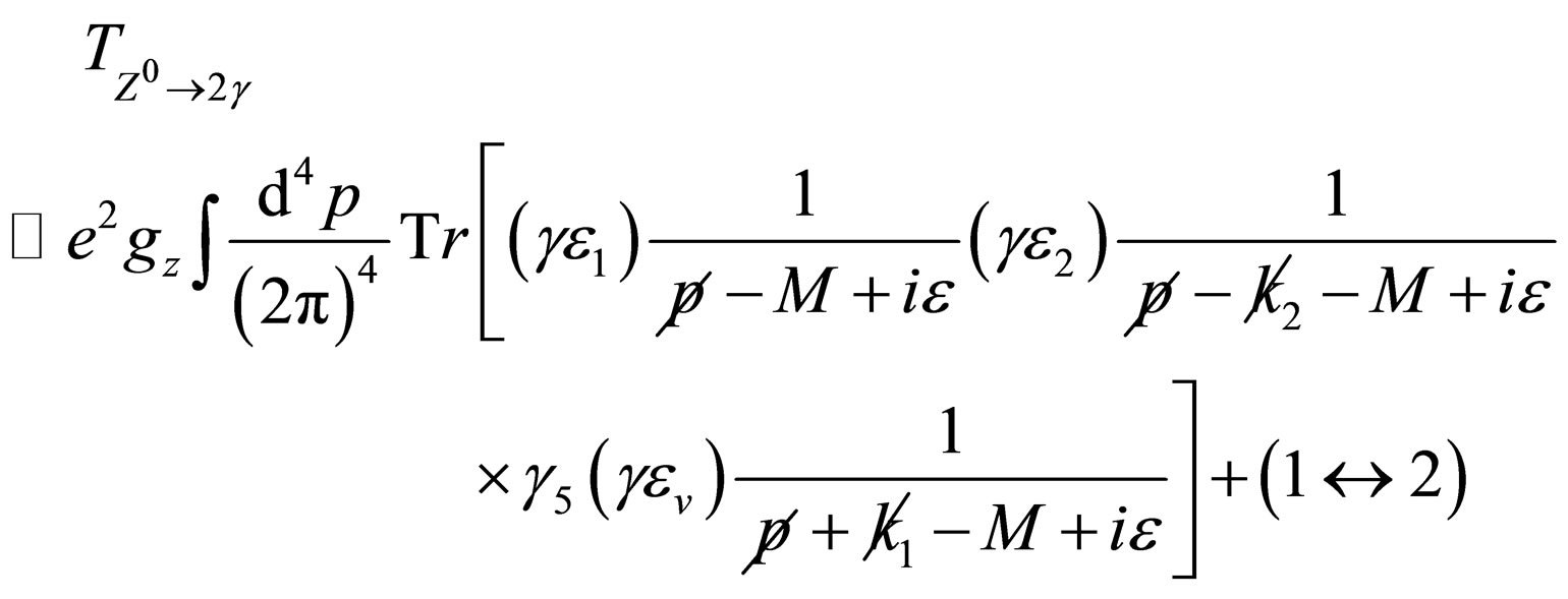(2.7)

where denotes the polarization vector of the boson. In this case, there seems to be an apparent linear divergence in Equation (2.7), and therefore one may have to worry about the renormalization procedure. Below is the field theory textbook description in order to derive the anomaly equation in four dimensions [1,2]. First, one defines the amplitude in Equation (2.7) as

(2.8)

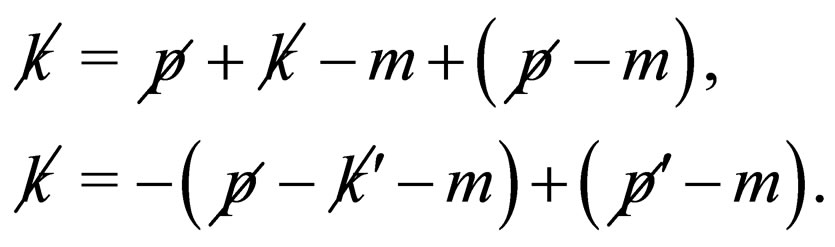
In this case, one says that the amplitude has an ambiguity which can be expressed in terms of an arbitrary momentum a. Using a mathematical identity, one can find the following equation [1,2,8]

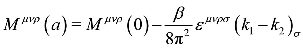(2.9)

where a is chosen as. The second term in the right hand side corresponds to the surface term which becomes finite as shown above. Here, can be determined so that the gauge condition can be satisfied. This just corresponds to the anomaly equation.

Now, the important point is that the divergent terms are still there, according to the proof of the chiral anomaly. Namely, the shift of the integration variable induces the additional term which is finite, but one cannot erase the divergence of the amplitude (there are still linear and logarithmic divergences). What does this physically mean? This clearly indicates that the anomaly equation has nothing to do with physical observables, and therefore there is no violation of the conservation law.

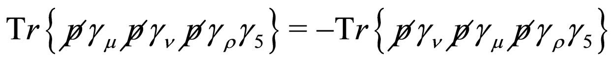
In reality, as we discuss below, the triangle diagrams with the axial vector current coupling do not have any divergences. It is quite unfortunate that people do not care for the infinity of the amplitude when they prove the anomaly equations, and this is somewhat a mystery why people have been accepting the mathematical game in the triangle diagrams even though the amplitudes have no infinity. Obviously, the disappearance of the apparent linear divergence is quite well known from the calculation of the fermion self-energy diagrams which have just the same type of the linear divergence, and this is, of course, due to the fact that the linear divergence term should vanish due to the parity consideration. Further, if one carries out the T-matrix evaluation properly, then one can easily notice that the linear divergent term vanishes to zero simply because of the Trace evaluation, and thus the vanishing of the linear divergent term is proved before one worry about the infinity in the momentum integrals.

It should be noted that good old physicists must have known that the triangle diagrams do not have any divergences at all. Unfortunately, however, theoretical frontier physics is often controlled by imprudent and disconcerted physicists, and once it is accepted by majorities of these physicists, then it takes always quite long time to correct this wrong frontier physics to a right direction of modern physics, sometimes, more than 50 years, like the theory of the spontaneous symmetry breaking physics [6].

3. Process

Here, we discuss the physical processes which involve the axial vector coupling with vector bosons. In fact, if we include the weak interactions, then the triangle diagrams with the axial vector coupling should be connected to the physical observables. Namely, there is a possible decay process of a weak boson into two photons, that is,. This decay process is forbidden due to the Landau-Yang theorem as far as one stays in the electromagnetic interactions where the theorem is proved [10, 11]. However, the weak interaction certainly allows its decay due to the parity non-conservation, and this is just the triangle diagram involving the axial vector coupling.

3.1. T-Matrix Evaluation

We can carry out the calculation of the Feynman diagrams which correspond to the decay into two photons (see Equation (2.7)), and we show that the triangle diagrams with the axial vector coupling have neither linear nor logarithmic divergences. This is proved without any regularizations, and the total amplitude of decay process is indeed finite. Here, we briefly explain the T-matrix evaluation since the calculations in detail are given in [12].

3.1.1. Linear Divergence

First, we show that the linear divergence should vanish completely because of the following equation

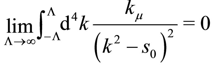(3.1)

which is just the same integration of the linear divergence appearing in the fermion self-energy diagrams. In fact, the fermion self-energy can be written as

(3.2)

where the last integral term is, of course, set to zero due to Equation (3.1), and the first term in the last equation is just the well-known fermion self-energy contribution. This fermion self-energy is well renormalized into the mass and the wave function, and in fact, this scheme is consistent with the Lamb shift energy.

In reality, however, the apparent linear divergence vanishes to zero before the momentum integration. This can be easily proved since the corresponding Trace evaluation of the T-matrix in Equation (2.7) becomes

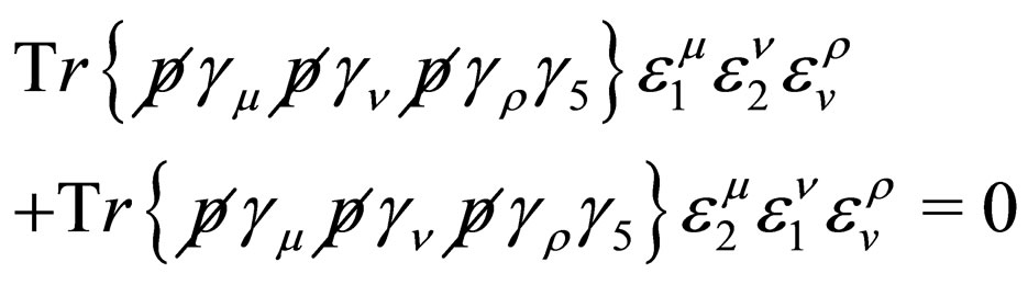(3.3)

where we made use of the identity equation

.

Therefore, the linear divergence disappears in Equation (2.7) before carrying out the momentum integral.

3.1.2. Logarithmic Divergence

Here, we should also note that the logarithmic divergence in Equation (2.7) is proved to vanish to zero exactly due to the Trace evaluation, and the detailed calculations are given in [12].

3.2. Branching Ratio of Decay

The finite term of the T-matrix for the process can be written as

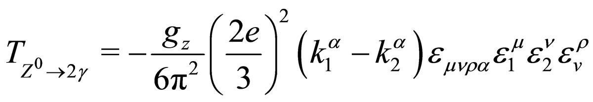(3.4)

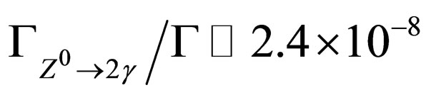
where the top quark state is taken as the intermediate fermions [12]. In this case, one can evaluate the branching ratio of the decay rate and find

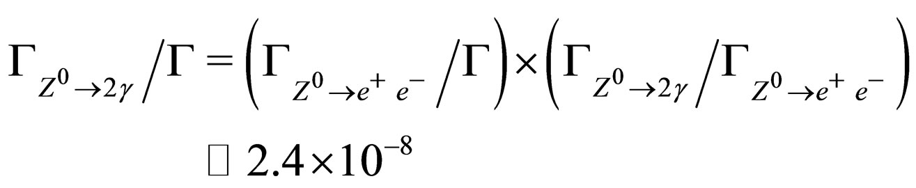(3.5)

where the experimental value of is used. Now, the present experimental upper limit of the branching ratio in this decay is given as [13]

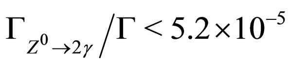(3.6)

which is still consistent with zero decay rate. This shows that the theoretical value of the branching ratio is, in fact, three orders of magnitude smaller than the present upper limit of the observation, but we believe that it should be measurable even though photon with around 45 GeV energies should be quite new to the present experimental detectors.

4. Anomaly in Schwinger Model

In the Schwinger model [5], the chiral anomaly property is well evaluated since all the equations can be obtained analytically. Here, we first review the procedure of obtaining the anomaly equation in the Schwinger model [4] since the anomaly equation represents the property of the vacuum state of the Schwinger model [14]. Then, we show that we can calculate the exact value of the chiral charge without any regularization, and the exact value of the chiral charge does not agree with the regularized chiral charge. Therefore, the anomaly equation is the artificial result of the regularization, and it is not a physically meaningful equation at all.

4.1. Chiral Charge of Schwinger Vacuum

The Schwinger model is the two dimensional QED with massless fermions and its Lagrangian density can be given as

(4.1)

where. After the field quantization, we can calculate the charge and the chiral charge of the vacuum state in the Schwinger model. In this case, we know that the charge of the vacuum state becomes infinity since we count the number of the negative energy particles. In order to obtain the finite number of the charge, we can employ the function regularization. In this case, the regularization can be done in accordance with the large gauge transformation. Therefore, we obtain the regularized charge and chiral charge as

(4.2)

(4.3)

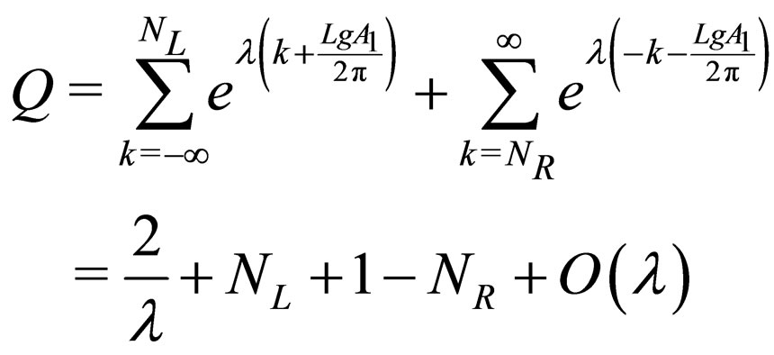
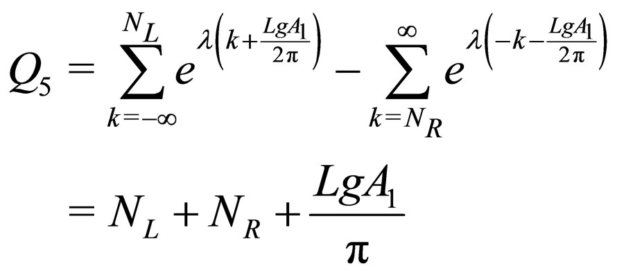
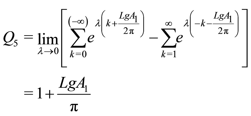
where denotes the vector field which only depends on time, and is an infinitesimally small number. The and denote integers which characterize the vacuum state for the left and right mover fermions. Since the physical vacuum must have zero charge, we can set. Therefore, we can write the chiral charge as [4]

(4.4)

where we set. Now, the important point is that the regularized chiral charge is described by, and therefore it should depend on time. This means that the chiral charge of the Schwinger vacuum state is not conserved any more, in contrast to the situation before the regularization. It is now easy to prove that Equation (4.4) leads to Equation (1.2).

Until now, this result of Equation (4.4) is taken as the indication that the conservation law of the axial vector current is violated due to the regularization, and people believe that it should give rise to some physical effect. However, we should here note that the chiral charge of the vacuum state has no divergence in contrast to the vacuum charge, and in this respect, there is no need of the regularization at all. In fact, from the definition of the chiral charge, we can see that the value of must be some integer value whatever physical conditions we impose on the system. Indeed, we can easily calculate the exact value of the in the vacuum state and finds as will be seen below. Here, we note that the Schwinger vacuum state has two fold degeneracy as indicated by and this is not resolved in this model. However, we do not discuss this degeneracy of the vacuum state since it is not relevant to the present discussion.

4.2. Exact Value of Chiral Charge in Schwinger Vacuum

In order to explain the exact value of the chiral charge in the Schwinger mode, we should first start from the quantized Hamiltonian of the Schwinger mode where the fermion field is quantized as

(4.5)

where and denote the creation and annihilation operators. In this case, the Hamiltonian of the Schwinger model becomes

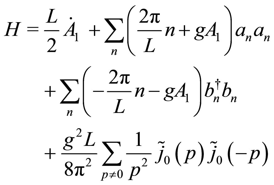(4.6)

where we take the Coulomb gauge fixing of. The current denotes the momentum representation of the fermion currents, and can be written

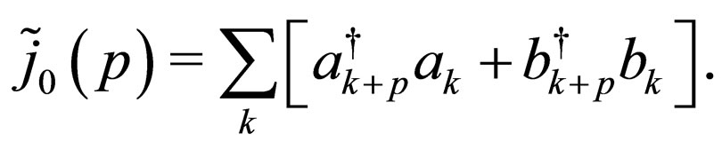(4.7a)

Also, the axial vector current in momentum representation is written as

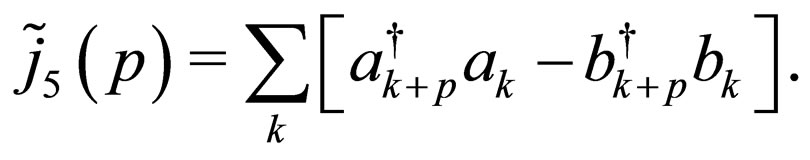(4.7b)

In this case, the chiral charge of the vacuum state which is filled with negative energy particles can be easily calculated as

(4.8)

where we have made no regularization, and this is just the exact result. On the other hand, as we show above, the regularized chiral charge is written in Equation (4.4)

which is different from the exact result. Now we can clearly see that the regularized chiral charge does not agree with the exact value of the chiral charge of the vacuum state, and therefore the regularization induces something unphysical. In fact, the chiral charge must be some integer value, but the induced value of the regularized charge is not an integer. Therefore, the axial vector current conservation is always valid, and there is no violation at all. This clearly states that the regularization cannot change the conservation law in quantum field theory. Or in other words, we should always be careful when we employ the regularization method, and the regularization scheme should be applied to the system such that the basic conservation law must be kept invariant. In addition, we should not make any regularization for the physical quantity which has no divergence. In the context of the Schwinger model, the regularization can be done for the charge since it is divergent, but not for the chiral charge. Concerning the charge of the vacuum, does not depend on time even if we use the gauge invariant regularization, and this is indeed shown in Equation (4.2).

4.3. Zero Mode in Schwinger Vacuum

It is well known that the Schwinger model can be bosonized, and in this case, the zero mode is related to the chiral charge [4]. Here, we should examine whether the zero mode can be found in the Schwinger vacuum state or not. Now, we see that the vacuum energy can be written as

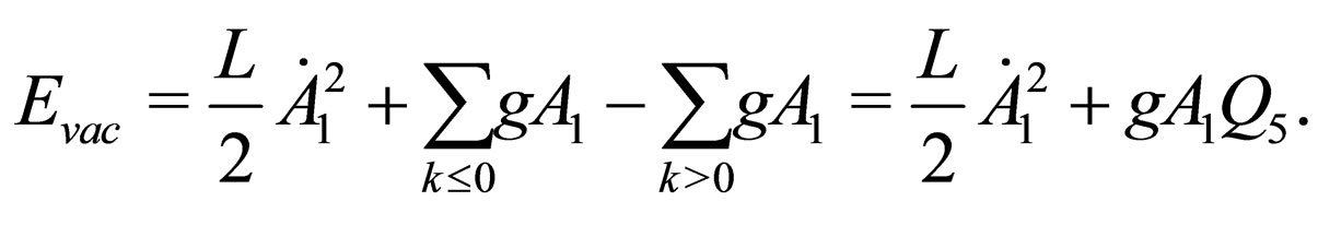(4.9)

Therefore, if one identifies the zero mode of the boson fields and its conjugate field as

(4.10)

then one can rewrite the vacuum part of the Hamiltonian as

(4.11)

which is indeed the zero mode Hamiltonian of the boson field. Therefore, the Schwinger model is bosonized properly since there is the zero mode part in the boson Hamiltonian. The basic point is concerned with the degree of freedom for the zero mode, and in fact, the gauge field of plays this role for the zero mode field in the bosonized Hamiltonian. In this respect, there is no need of the chiral anomaly from this point of view. This is in contrast to the massless Thirring model which has an intrinsic problem of the proper bosonization since the massless Thirring model has no degree of freedom which corresponds to the zero mode [6].

4.4. Summary of Anomaly Problem

The chiral anomaly problem is one of the most serious theoretical syndromes, and it means that they are mathematically correct, but physically incorrect. The regularization is a mathematical tool, and the procedure of its application to physics is mathematically correct, but the anomaly equations are physically incorrect since they are discovered when the regularization method is applied to the systems which have no divergence as a physical process. It is very unfortunate that there are too many examples of “mathematically correct, but physically incurrect” such as the spontaneous symmetry breaking physics, general relativity, field theory path integral and so on [6]. We should understand nature in depth, both mathematically and physically, and we have to connect the mathematics to physical observables, and this connection is real physics which is always extremely difficult indeed.

5. Renormalization Scheme in QED

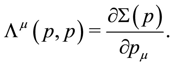
In this section, we briefly explain the essential point of the renormalization scheme. In particular, we show that the self-energy of photon is not needed in the renormalization procedure since there is no relevant physical process which can make use of the renormalized wave function of the photon self-energy, in contrast to the fermion self-energy case. The important point is that the vertex correction corresponds to the Feynman diagram in which the external electromagnetic field couples to the intermediate fermion state in the fermion self-energy diagram. On the other hand, the triangle diagrams correspond to the Feynman diagram in which the external vertex of couples to the intermediate fermion or antifermion states in the photon self-energy diagram. Both of the procedures in the renormalization scheme are quite similar to each other, but the vertex correction has the logarithmic divergence which should be absorbed into the renormalized wave function of fermions while the triangle diagrams have no divergences at all, and thus there is no need of the renormalization procedure for the photon self-energy case as long as we aim at producing physical observables.

5.1. Renormalization of Fermion Self-Energy

Before going to the discussion of the renormalization procedure of the photon self-energy, we first explain the renormalization procedure of the fermion self-energy case which can be directly related to the vertex correction. The self-energy of fermion can be written as

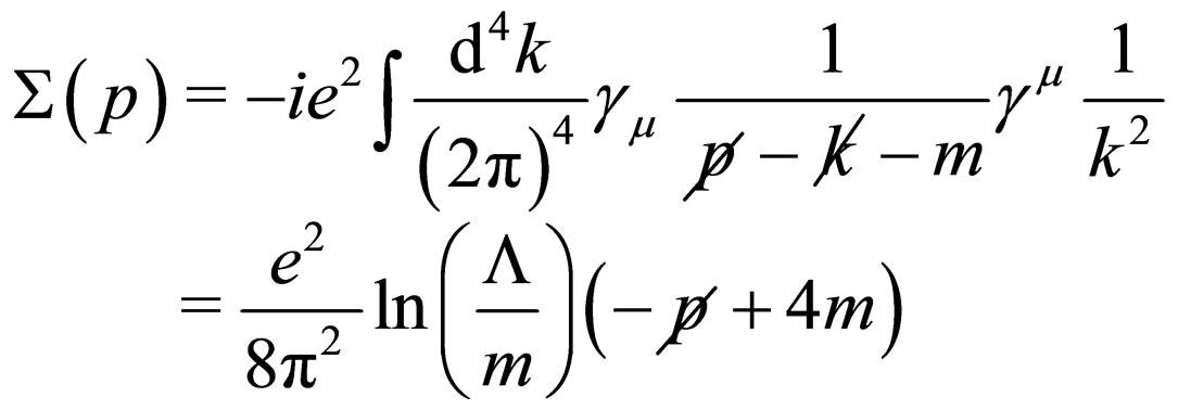(5.1)

where denotes the cutoff momentum. It is, of course, clear that this contribution alone is not a physical observable. However, if one calculates the vertex correction which is indeed a physical process, then one realizes that one must make use of the logarithmic divergence of the fermion self-energy contribution such that the logarithmic divergence of the vertex correction can be completely canceled out by the wave function renormalization arising from the fermion self-energy diagram. In fact, the total Lagrangian density of free fermion together with the fermion self-energy part can be written as

(5.2)

where is defined as

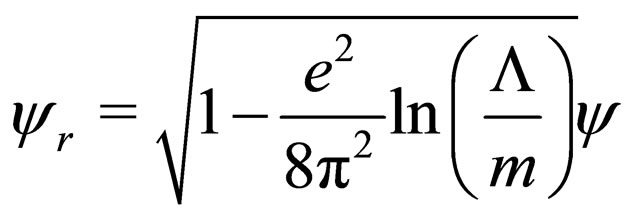(5.3)

Here, we only write the term since the mass term is not relevant in the present discussion. Now we can calculate the vertex correction as

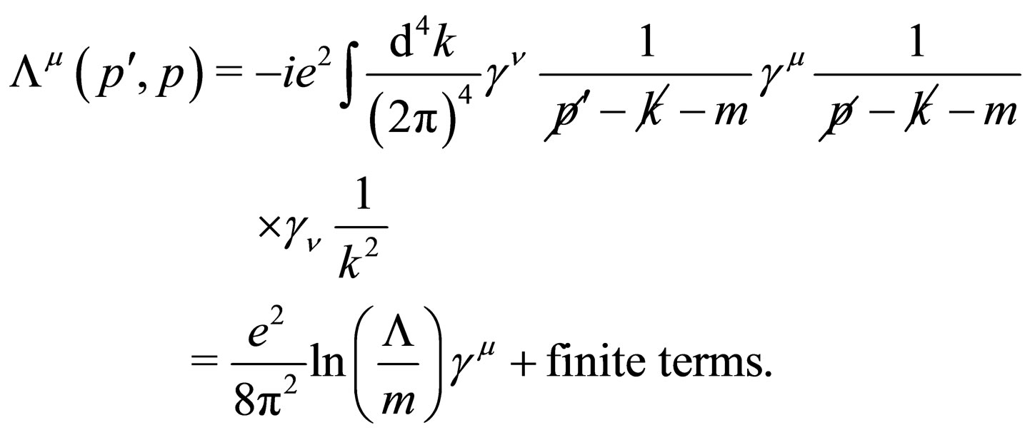(5.4)

Therefore, the total interaction Lagrangian density can be written as

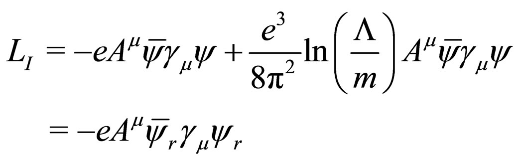(5.5)

where the logarithmic divergent part can be completely absorbed into the renormalized wave function.

5.2. Renormalization of Photon Self-Energy

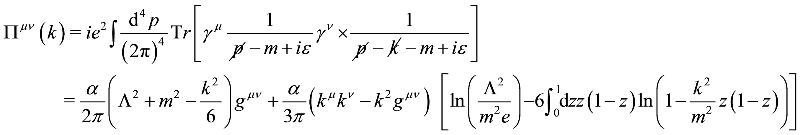
The self-energy of photon can be easily calculated, and the divergent terms of the vacuum polarization tensor can be written as

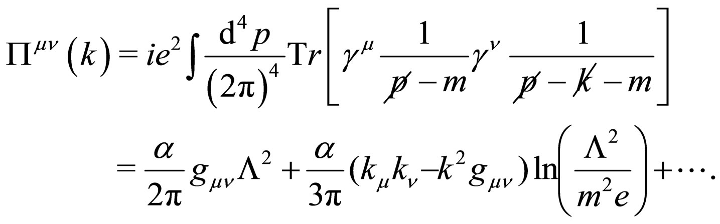(5.6)

Now it is obvious that the self-energy of photon itself is not a physical observable. Further, the important point is that the vacuum polarization diagrams are never used for the renormalization scheme of evaluating physical observables in the triangle diagrams, in contrast to the fermion self-energy case.

5.3. Triangle Diagrams with Two Photons

In analogy with the vertex correction, we should consider the triangle diagrams which can be viewed as an external vertex coupled to the photon self-energy diagram. The vertex which couples to fermion or anti-fermion can be written in the following functions,

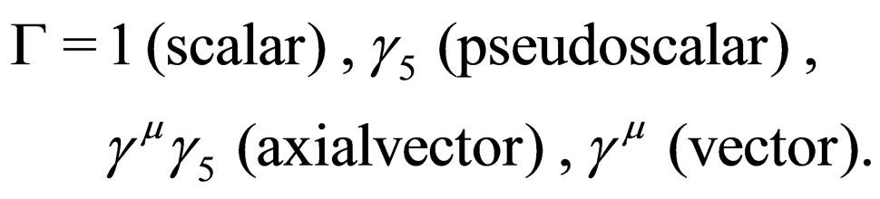(5.7)

However, as we show explicitly in Appendix B, the calculated results of these T-matrices of the triangle diagrams involving two photons have no divergences and the physical processes with the vacuum polarization diagrams are all finite. This means that there is no necessity of considering the photon self-energy into the renormalization scheme.

It is surprising that this fact is indeed overlooked by experts. We should note here that the calculations of the triangle diagrams are not so easy, but if smart graduate students spent a half year, then they should be able to find that all of the triangle diagrams with any vertices coupled to fermions should not have any divergences at all.

5.4. Lamb Shift Energy

The renormalization scheme is, by now, well understood since the logarithmic divergence only appears in the vertex corrections due to the photon propagation. However, the Lamb shift is still very difficult to understand since it has a logarithmic divergence, even though it is a physical observable. At least, Bethe’s treatment of the Lamb shift energy must have some intrinsic problems since it cannot avoid the logarithmic divergence in his treatment [15]. Even though his treatment is non-relativistic, the hydrogen atom wave function can be well evaluated by the non-relativistic calculation. Therefore, the basic problem of the logarithmic divergence in the Lamb shift energy may well be related to some other fundamental physical reasons, unles one can prove that the relativistic treatment of the Lamb shift energy is finite.

The basic difficulty must come from the fact that the Lamb shift energy is evaluated outside the Fock space of the renormalization scheme, that is, the bound states cannot be found in the Fock space of free fields. This should give rise to a difficulty since it cannot be handled in terms of the wave function renormalization. Indeed, the Lamb shift is concerned with the mass term of the fermion self-energy contribution. However, the logarithmic divergence is still there in the Lamb shift calculation, even though it is a physical observable. This situation is far from being satisfactory, but we do not find any direction of solutions at the present stage.

5.5. Specialty of Photon Propagations

As we understand by now, the only serious divergence we have in the calculation of physical observables is concerned with the vertex corrections due to the propagation of photon, since there is no divergence in the vertex corrections due to the propagation of the massive vector boson as discussed in Section 6. It turns out that this logarithmic divergence arises from the choice of the propagator of photon

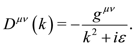(5.8)

This is, of course, the standard photon propagator. The problem is that we cannot employ the following propagator

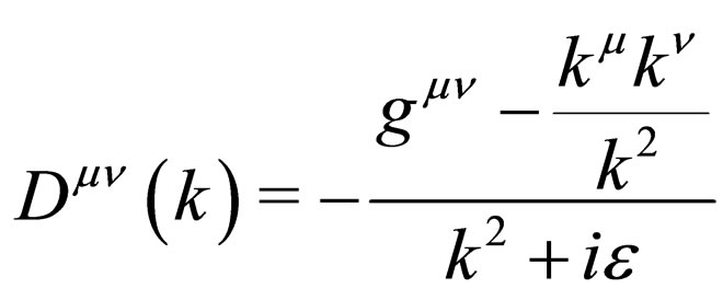
since it is not allowed because of the infra-red singularity in the numerator of the propagator. Therefore, we have to choose the photon propagator of Equation (5.8) to carry out the calculations in terms of the covariant formulation. This propagator leads to the logarithmic divergence of the vertex corrections by photon propagation, even though the vertex corrections are physical observables. At present, we do not find any other solutions than the renormalization procedure which makes use of the self-energy of fermions as discussed above.

It should be interesting to note that the vertex corrections by the photon propagation contain the infra-red singularity of [16]. Up to the present stage, we have neglected this infra-red singularity since it is consistent with experiments. However, this does not mean that we have understood the problem theoretically. On the other hand, the renormalization scheme of the massive vector boson propagations does not have any divergences at all in the vertex corrections, and in this sense, it is well understood as we discuss below.

6. Renormalization Scheme in Weak Interactions

Here we discuss the renormalization scheme in which fermions are affected by the weak vector bosons. In this case, we should first evaluate the propagator of the massive vector bosons since the new condition of the polarization vector is obtained. Then, we calculate the fermion self-energy and vertex corrections due to the massive weak boson propagator which has a right behavior at the high momentum region, in contrast to the old propagator of the massive vector boson. We see that the fermion self-energy has a logarithmic divergence while the vertex corrections are all finite, that is, there exist neither quadratic nor logarithmic divergences in the T-matrices of the vertex corrections. Therefore, there is no need of the renormalization procedure for the vertex from the massive vector boson propagations. Before going to the renormalization scheme, we should first evaluate the propagator of the massive vector boson in a correct way.

6.1. Propagator of Massive Vector Fields

At present, most of the field theory textbooks employ the following propagator of the massive vector boson

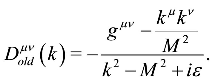
However, as we show below, this is not a right propagator for the massive vector boson. This mistake is basically due to the fact that the solution of the constraint equation for the polarization vector of Equation (C.11) was not used for the determination of the propagator. As we prove in Appendix C, the Lorentz condition

always holds for the massive and gauge bosons as well since it is the result of the equation of motion for the polarization vector. Here, we evaluate the propagator of the massive vector field. First, starting from the S-matrix expression, we can calculate the second order perturbation energy for the bosonic part. In this case, we insert the expression of Equation (C.10) into the T-product of, and the calculation can be carried out in a straight forward way. The result becomes

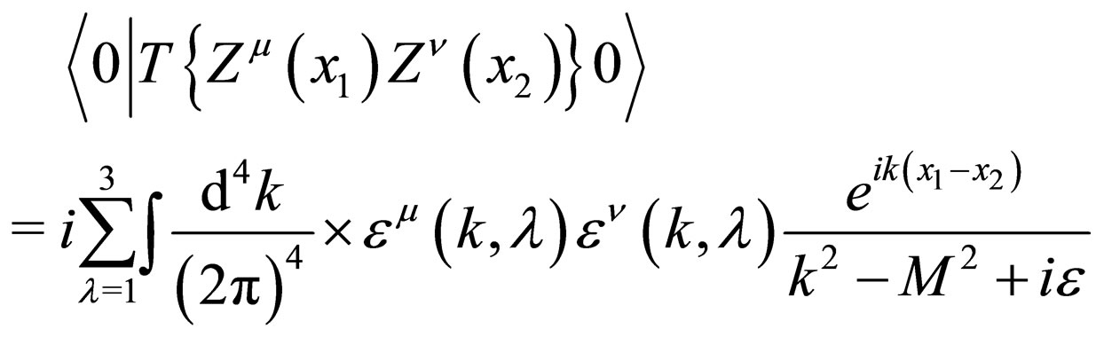(6.1)

where denotes the vacuum state of massive boson Fock space. After the summation over the polarization states, we find the following shape for

as

(6.2)

which satisfies the Lorentz invariance and the condition of the polarization vector. It is only this solution that is possible for the free massive vector field. Therefore, we see from Equation (6.2) that the right propagator of the massive vector boson should be given as

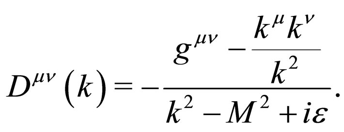(6.3)

Here it may be important to note that the polarization vector should depend only on the four momentum, and it cannot depend on the boson mass at this expression. Later on, one may replace the term in the numerator of Equation (6.3) by in case the vector boson is found at the external line. But in the propagator, the replacement of the term by is not allowed.

6.2. Fermion Self-Energy by Weak Bosons

The interaction Lagrangian density for the boson and electron can be written as

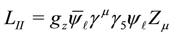(6.4)

In this case, the self-energy of fermion due to the weak boson can be written as

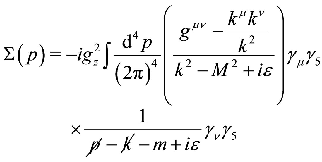(6.5)

which can be easily evaluated to be

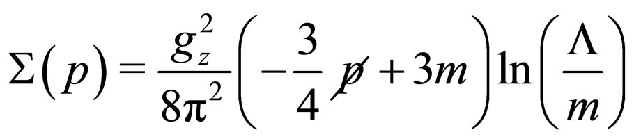(6.6)

where denotes the cutoff momentum. It is, of course, clear that this contribution alone is not a physical observable.

6.3. Vertex Corrections by Weak Bosons

Now we can calculate the vertex correction of electromagnetic interaction due to the boson as

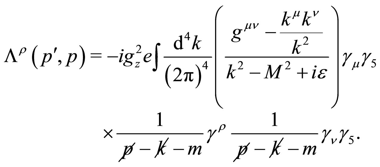(6.7)

This can be easily calculated, and below we discuss the results in terms of the apparent logarithmic divergent term and the mass dependent term, respectively.

6.3.1. No Divergence

First, the apparent divergent terms in Equation (6.7) can be written as

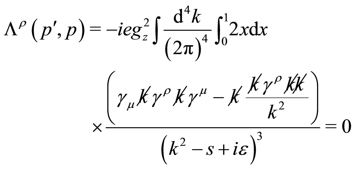(6.8)

where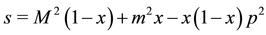. Therefore, there is no logarithmic divergence for the vertex correction. This is quite interesting since the vertex correction is related to physical observables and thus the result should be obtained as a finite number. In addition, the self-energy of fermions has logarithmic divergences, but this time it is simply useless because the vertex correction has no divergence.

6.3.2. Electron g – 2 by Z⁰ Boson

The finite part of the vertex correction due to the Z⁰ boson can be easily calculated and, therefore, the electron g – 2 should be modified by the weak interaction to

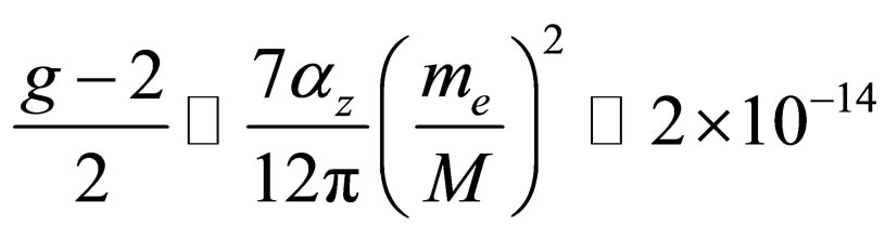(6.9)

where 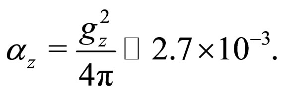This is a very small effectand therefore, it is consistent with experiment. We should note that, if we employed the standard propagator of the massive vector boson as given in the field theory textbooks [9], then we would have obtained a very large effect on the electron, even if we had successfully treated the problem of the quadratic and logarithmic divergences in some way or the other, by renormalizing them into the fermion self-energy contributions. This strongly suggests from the point of view of the renormalization scheme that the propagator of the massive vector field should be the one given by Equation (6.3).

6.3.3. Muon g – 2 by Z⁰ Boson

Here, we should also give a calculated value of the muon due to the Z⁰ boson since it is just the same formula as Equation (6.10) except the mass of lepton. The result becomes

(6.10)

which is much larger than the electron case. This is, however, still too small to be observed by the muon experiments at the present stage.

6.4. Ward Relation

Here, we should make a comment on the Ward relation [17]. This relation starts from the following equation

(6.11)

which is always valid as an operator equation, and the Ward relation is written as

(6.12)

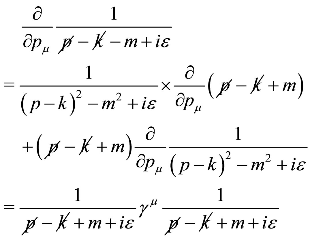
Since the self-energy of fermion is defined in Equation (5.1), the Ward relation corresponds to taking the first term in Equation (6.11) before the momentum integrations. The second term of Equation (6.11) should contribute to the vertex corrections, though it depends on the shape of the integrand. Here, one should be careful for the validity of Equation (6.12) since one normally makes use of the following free dispersion relation

(6.13)

In the evaluation of the self-energy of fermion, we replace the term by in the denominator of the fermion self-energy calculations. In this case, there is no guarantee that Equation (6.12) holds true since one has neglected the second term in Equation (6.11) to calculate the self-energy of fermion before the differentiation with respect to. Therefore, one should carefully evaluate the vertex corrections without referring to the Ward identity. In fact, the validity of Equation (6.12) can be proved for the logarithmic divergence in the evaluation of the vertex corrections for the photon propagation. However, we believe that it is simply accidental because, this is not valid any more for the vertex corrections from the massive vector boson propagation as one can clearly see it in Equation (6.8).

In this respect, we see that identity equations are sometimes useful for checking mathematical formula, but we should be very careful for applying the identity equation to physical processes. This is, of course, clear since there should be always many severe conditions when we apply the mathematical equations to physical processes. In fact, it is very rare that identity equations can be applied to physics without making mistakes. The Ward relation and the gauge condition are good examples in which we can easily make mistakes.

7. Conclusions

We have critically reviewed the anomaly problem in four and two dimensional QED and have clarified that the anomaly equation is a spurious equation and it has nothing to do with real physics. However, there is one thing which is still unclear, that is, why people believed that a new term which is derived from the regularization can be a new physical quantity even though it violates the conservation law. This conservation law of the axial vector current for massless fermions is derived from the symmetry argument, and this symmetry is, of course, kept valid after the field quantization. But it is accepted that this conservation law can be violated by the regularization scheme as an operator form. This means that the regularization scheme is something which is beyond our normal understanding of field theory. This is the very point we cannot understand up to now, and this blind belief in the regularization scheme spread over most of the physicists. This jeopardizes a sound scientific thinking, and the chiral anomaly physics must be one of the biggest stains in modern field theory.

Further, we have discussed the renormalization schemes in QED and weak interactions so as to clarify the present understanding of the renormalization procedure. The renormalization scheme in QED is basically a review since it has a good understanding of the renormalization. However, the renormalization scheme in weak interactions should be examined more carefully since the propagator of the massive vector boson should be modified to a correct expression. This leads to the new scheme in which the vertex corrections are found to be finite, and thus there is no need of the renormalization. This is somewhat similar to the situation of the triangle diagrams which have no divergence, and thus no renormalization procedure is necessary for the vacuum polarization diagrams. In this respect, the renormalization scheme becomes much less ambiguous than before, and we should try to understand further what kind of physical observables we can calculate by the renormalization schemes.

REFERENCES

Appendix

1. Regularization

It should be worthwhile clarifying what the regularization means in physics. Mathematically, most of the regularizations are clear, except the dimensional regularization which has made crucial mistakes in using mathematical formula.

1.1. Cutoff Momentum Regularization

The simplest and most reliable regularization method is known in terms of the cutoff in which the integral of the momentum can be set to

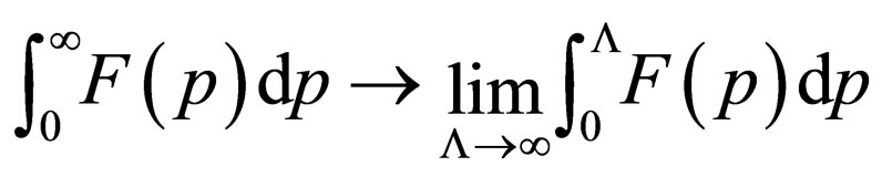(A.1)

where is called the cutoff momentum. This has a good physical meaning since the integral over the momentum corresponds to the summation of all the possible states in the Fock space of the field theory one considers. Therefore, the introduction of the cutoff momentum means that the maximum number of the states in the field theory model is now fixed to with L the box length. In this sense, if the cutoff momentum is much larger than any scales in the model field theory, then one can reliably obtain the calculated results under the condition that the physical observables should not depend on the.

1.2. Pauli-Villars Regularization

Now, another popular regularization must be the PauliVillars regularization [18]. This is rather simple and it makes the divergent integral to the convergent integral in the following way

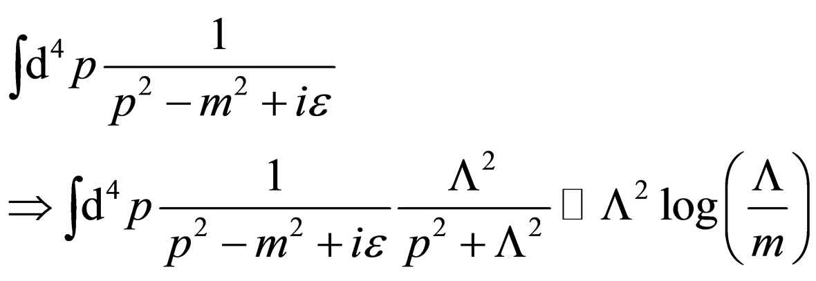(A.2)

which is indeed convergent. However, if we make the to infinity, then we can get back to the infinity as the original integral (l.h.s. of Equation (A.2)) indicates. Therefore, there is no point to employ the Pauli-Villars regularization.

1.3. -Function Regularization

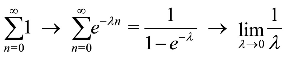
The third example can be the function regularization [4], and in this case, the summation can be replaced in the following way

(A.3)

where the original infinity is certainly kept in terms of. In this respect, the apparent infinity can be expressed in terms of some finite numbers and the original infinity can be recovered when the parameter is set to zero or infinity depending on the regularization. Mathematically, the regularizations we discuss here can satisfy the important condition that the original divergence can be recovered by setting the parameters to zero or infinity.

1.4. Dimensional Regularization

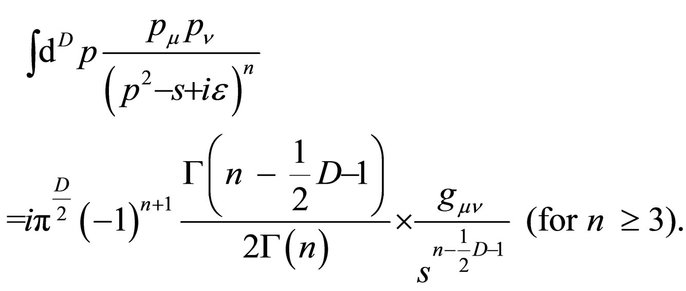
Finally, we discuss the dimensional regularization which is, however, quite different from other examples [19,20]. It cannot satisfy this most important mathematical condition that the original infinity should be recovered when we set the parameter to zero or infinity. In the dimensional regularization, the parameter is since they replace the integral dimension from 4 to. In this case, one uses the following integral formula

(A.4)

The important point is that Equation (A.4) is only valid for, and this is the very strict condition. In fact, if one applies Equation (A.4) to the calculation of the photon self-energy diagram (), then one cannot recover the quadratic divergence in the dimensional regularization even when one sets the value of the parameter to infinitesimally small. What does this means? It indicates that the dimensional regularization must be mathematically incorrect for the quadratic and higher divergent evaluations. For the case of the logarithmic divergence, the dimensional regularization can give a correct result, though the divergence level is somewhat different from the normal regularizations. In this respect, the dimensional regularization is a useless regularization method.

1.5. Summary of Regularization

To summarize, we see that the regularization is simply a mathematical tool, and if we employ some regularization method and obtain some equations which violate the conservation law, then we should realize that the regularization method we use must be inappropriate for the case we treat. In terms of physics, the regularization cannot be more than the mathematical tool, and we have to always think over in depth what are physically interesting observables. The regularization may present some way of finding interesting physical observables by making infinite quantities to finite numbers for a while, and this finite numbers may enable us to understand some phenomena in physics in a better way.

2. Gauge Invariance

In connection with the anomaly problem, the gauge condition is closely related to the derivation of the anomaly equation. Therefore, we should clarify the situation of the gauge invariance in QED since there is a serious misunderstanding among some of the educated physicists concerning the gauge invariance of the calculated amplitudes which involve the external photon lines. Their argument is as follows. The polarization vector is gauge dependent and therefore the calculated results must be kept invariant under the transformation of

.

However, this condition is unphysical since we already fixed a gauge (for example, Coulomb gauge fixing of) before the field quantization. The gauge invariance of the S-matrix evaluation is guaranteed as far as the fermion current is conserved, which is always satisfied in the perturbation calculation.

2.1. Vacuum Polarization Tensor

The best example can be found in the vacuum polarization tensor. People believe that the following gauge condition should be satisfied [16]

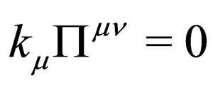(B.1)

which is required from the above argument of the gauge condition as well as some incorrect mathematical identity equation [21]. However, as one can easily examine, this is a wrong equation. In fact we can easily calculate and write the result of the standard calculation of the vacuum polarization tensor as [22]

(B.2)

where denotes the cutoff momentum. There is no way that the first term of the right hand side can satisfy the gauge condition of Equation (B.1). Namely we find

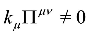(B.3)

and therefore, Equation (B.1) cannot be satisfied by the vacuum polarization tensor. People believed Equation (B.1) should hold true, basically because of the mathematical mistake due to the wrong replacement of the integration variables in the infinite integrals [6,21]. Since then, the gauge conditions are imposed by hand on the amplitudes which have some external photon lines. However, it should be noted that the same type of the calculations of the vacuum polarization was done a long time ago by Heisenberg and Euler [23,24] and they obtained the similar results as above including the quadratic divergence and logarithmic divergence as well. Even though their argument of the polarization process is not in the right direction in terms of the renormalization scheme [21], their calculations themselves are indeed correct.

2.2. Vacuum Polarization Tensor for Axial Vector Coupling

Here, we should check whether the gauge condition can be satisfied for other reaction processes or not. First, we should present an example of the vacuum polarization tensor which is induced by the axial vector current which couples to fermions as

In this case, the vacuum polarization tensor for the axial vector current can be written as

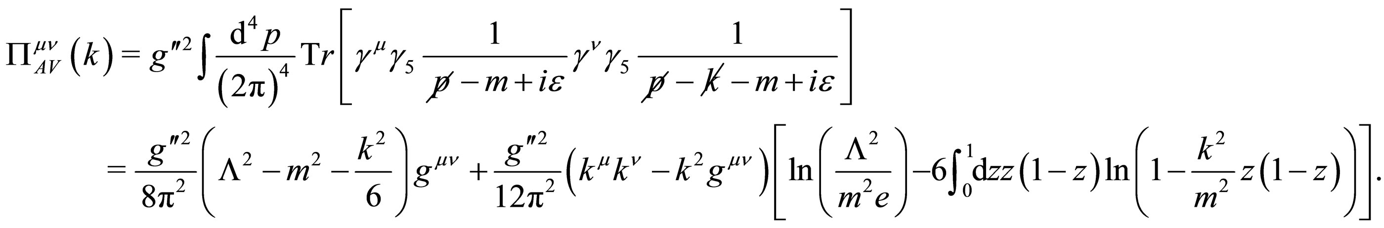(B.4)

This clearly shows that the axial vector current conservation is not related to the gauge condition since we have

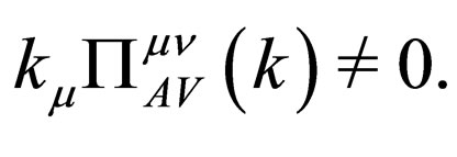(B.5)

On the other hand, the Compton scattering case is different and it can satisfy the gauge condition since there is no fermion loop in this calculation.

2.3. Compton Scattering

The Feynman amplitude of the Compton scattering can be written as

(B.6)

Therefore, we can check

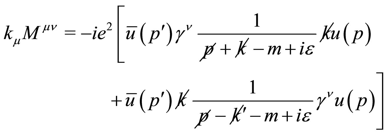(B.7)

Now, using some identities

and the free Dirac equations of

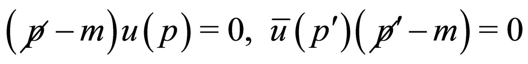(B.8)

we can easily prove

(B.9)

However, this is, of course, clear since the Compton scattering does not contain a loop diagram, and therefore the gauge condition, just corresponds to the conservation of the fermion current, and this can be easily seen since the initial and final fermion in the Compton scattering can satisfy the free Dirac equation. On the other hand, if the Feynman diagrams involve the fermion loop, then there is no reason that the gauge condition can directly correspond to the fermion current conservation since the free Dirac equation cannot be used.

2.4. Decay of

Among the Feynman diagrams that contain the fermion loop, the decay of the can satisfy the gauge condition. Now, the T-matrix of can be evaluated to be

(B.10)

Defining the amplitude as, we can prove

(B.11)

which is due to the anti-symmetric character of the tensor. This property is basically due to the interaction which generates the anti-symmetric nature of the invariant amplitude. In this respect, it is very special that the decay process satisfies the gauge condition, and it is not due to the nature of the electromagnetic interactions. This pion and nucleon interaction is, in fact, beyond QED, and it indeed involves the strong interaction. Since the strong interaction satisfies the parity invariance, the Feynman diagram of the decay process keeps the anti-symmetric nature, and thus the amplitude satisfies Equation (B.11), and this is, of course, accidental from the point of view of the gauge condition. This point can be clearly seen if we examine the reaction process of the scalar meson decay into two photons since the scalar interaction has the symmetric nature.

2.5. Decay of Vector Boson Z⁰ into

The T-matrix for the decay process is given in Equation (3.8)

(B.12)

Therefore we can define the amplitude as, we can now prove

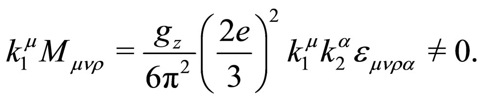(B.13)

Therefore, the gauge condition is not satisfied in the case of of decay process. This is, of course, clear since the interaction has a symmetric nature and therefore it is just opposite to the interaction.

2.6. Decay of Scalar Boson Φ into

Now, the T-matrix of can be evaluated to be

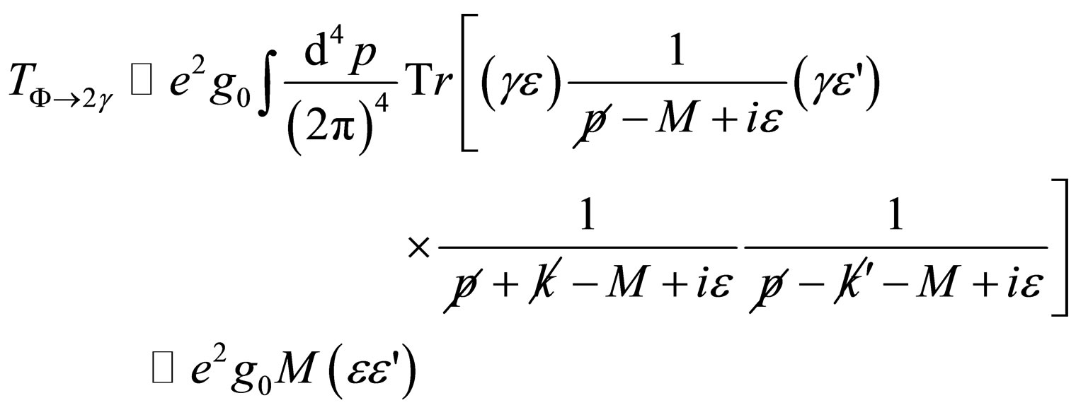(B.14)

where M denotes the nucleon mass, and is the coupling constant of interaction as described by. Defining the amplitude as 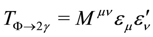, we can now prove

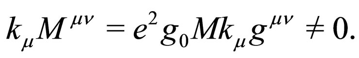(B.15)

Therefore, the gauge condition is not satisfied in the case of of decay process. This is, again, easy to understand since the scalar interaction has a symmetric nature and therefore it is opposite to the interaction.

It should be noted that there is no scalar meson in nature which decays into two photons. However, the similar type of the Feynman diagram becomes important when we consider the photon-gravity interaction. In fact, photon can interact with the gravitational field via loop diagrams which are essentially the same as the T-matrix given in Equation (B.14) [6]. In this respect, the T-matrix of Equation (B.14) can be considered to be a physical process.

2.7. Photon-Photon Scattering

The T-matrix of the box diagrams in the photon-photon scattering can be written as

(B.16)

where the energy of photon can be written as

at the center of mass system of two photons. The leading behavior of the finite terms in this T-matrix can be easily evaluated under the condition of and we write it in terms of which is defined as

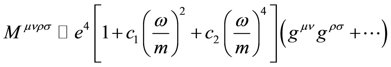(B.17)

where and denote some numerical constants. Therefore, it is clear that the gauge condition does not hold, and we have

(B.18)

It should be important to note that the apparent divergences can be completely cancelled out due to the kinematical cancellation by adding up three independent Feynman diagrams together, and the disappearance of the divergences is not due to the regularization [25].

2.8. Gauge Condition and Current Conservation

As we saw above, the serious mistake must be concerned with the confusion between the gauge conditions and the current conservation. Somehow, people believed that the gauge condition should be directly connected to the current conservation [1]. Or in other words, the gauge condition of the Feynman amplitude (we denote it as) for some reaction process

(B.19)

should be identical to the current conservation of

(B.20)

This is, of course, a wrong statement, and the current conservation must hold true for any occasions while the gauge condition of Equation (B.19) is in some cases satisfied and in other cases not, depending on the reaction processes as we saw above. Basically, the current conservation cannot manifestly be traced in the Feynman amplitude of unless there are external fermion lines which can satisfy the free Dirac equation, and consequently can be related to the current conservation.

In this sense, the condition of the reaction amplitude involving the axial vector vertex of with its polarization vector

(B.21)

does not mean that the axial current conservation is violated. We have shown that the gauge condition of does not have any physical meaning, but the replacement of is even worse than the gauge condition since the axial vector coupling has nothing to do with the gauge theory. In this respect, the whole business of the anomaly equation is just the castle in the air.

2.9. Summary of Gauge Condition

To summarize, we see that the Compton scattering and decay process can satisfy the gauge condition, while other examples of the photon self-energy, the vacuum polarization for the axial vector current, the decay process, photon-photon scattering diagrams and decay process do not satisfy the gauge condition, and this is mainly because they have a fermion loop.

It is by now clear that the gauge condition of is physically a meaningless procedure. This is basically due to the fact that the Lorentz condition of is obtained from the equation of motion as explained in Appendix C. Therefore, this constraint equation cannot be taken as the gauge fixing condition, and thus the requirement of is physically a wrong procedure.

3. Lorentz Condition

Here, we clarify that the Lorentz condition of should be obtained from the equation of motion, and therefore it is more fundamental than the requirement of the gauge fixing condition.

3.1. Gauge Field of Photon

We write the Lagrangian density for the free gauge field as

(C.1)

with. In this case, the equation of motion becomes

(C.2)

Since the free photon field should have the following solution

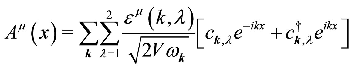(C.3)

we can insert this solution into Equation (C.2) and obtain the following equation for

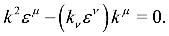(C.4)

This equation can be written in terms of the matrix equation for the polarization vector as

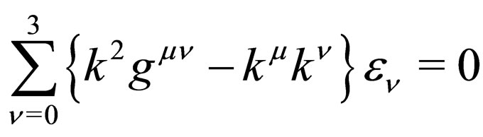(C.5)

where we write the summation explicitly. In order that the should have a non-zero solution, the determinant of the matrix should vanish, namely,

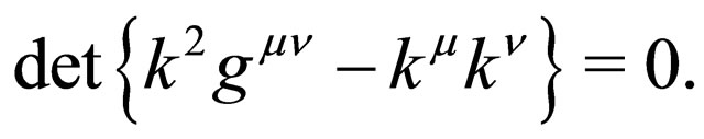(C.6)

Now it is easy to prove that is the only physical solution of Equation (C.6) since one finds

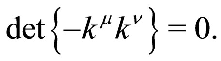
Therefore, putting the solution of into Equation (C.4), we obtain

(C.7)

which becomes the solution for the polarization vector. Here, we should note that this process of determining the condition on the wave function of is just the same as solving the free Dirac equation. Obviously this is the most important process of determining the wave functions in quantum mechanics, and surprisingly, this has been missing in the treatment of determining not only the massive vector boson propagator but also the photon propagator as well.

This constraint equation of Equation (C.7) is obtained from the equation of motion, and therefore it is more fundamental than the gauge fixing condition even though it is just the same equation as Lorentz gauge fixing condition. In this respect, the condition of should be always satisfied since it is derived from the equation of motion. As one can see by now, the gauge fixing condition is still left for use. In fact, if we take the Coulomb gauge fixing of, then we find which leads to the condition of. Therefore, we now see that the photon field has only two degrees of freedom which can be naturally obtained from the equation of motion and the gauge fixing condition.

In addition, one realizes that the Lorentz gauge fixing is not allowed in the free field gauge theory since the same equation of the Lorentz gauge fixing is already obtained from the equation of motion. Namely, it cannot give a further constraint on the polarization vector. In this respect, one sees that the Coulomb gauge fixing gives a proper condition on the polarization vector.

3.2. Massive Vector Fields

The massive vector field can be treated just in the same manner as above. We first write the free Lagrangian density for the vector boson field with its mass M

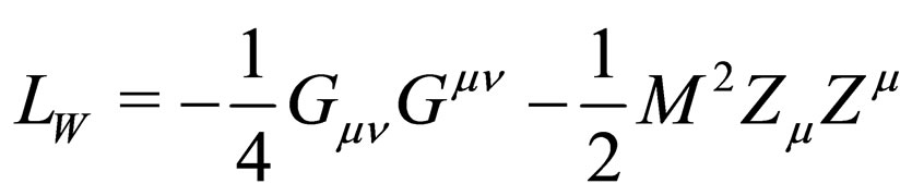(C.8)

with. In this case, the equation of motion becomes

(C.9)

Since the free massive boson field should have the following shape of the solution

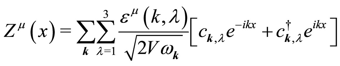(C.10)

we can insert this solution into Equation (C.9) and obtain the following equation for the polarization vector

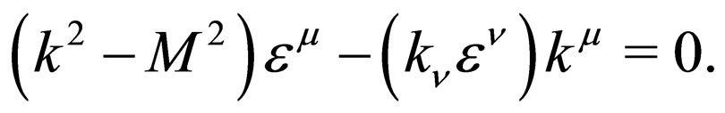(C.11)

In the same way as above, we can prove that

should hold, and this is the only physical solution of Equation (C.11). Therefore we obtain the following equation for the polarization vector

(C.12)

which should always hold. This is just the same equation as Lorentz gauge fixing condition in QED. However, there is no gauge freedom for the massive vector boson, and therefore the degrees of freedom of the polarization vector for the massive vector boson is three, in contrast to the gauge field. Even though the gauge field naturally requires the massless nature of the photon field, one should not claim that the number of the degrees of freedom of the photon field is a direct consequence of the massless nature.

REFERENCES

- C. Itzykson and J. B. Zuber, “Quantum Field Theory,” McGraw-Hill, New York, 1980.
- L. Ryder, “Quantum Field Theory,” Cambridge University Press, Cambridge, 1996.
- S. I. Adler, “Vertex in Spinor Electrodynamics,” Physical Review, Vol. 177, 1969, pp. 2426-2438. doi:10.1103/PhysRev.177.2426
- N. S. Manton, “The Schwinger Model and Its Axial Anomaly,” Annals of Physics, Vol. 159, No. 1, 1985, pp. 220-251. doi:10.1016/0003-4916(85)90199-X
- J. Schwinger, “Gauge Invariance and Mass,” Physical Review, Vol. 128, No. 5, 1962, pp. 2425-2429. doi:10.1103/PhysRev.128.2425
- T. Fujita, “Symmetry and Its Breaking in Quantum Field Theory,” 2nd Edition, Nova Science Publishers, New York, 2011.
- K. Nishijima, “Fields and Particles,” W. A. Benjamin, Inc., San Francisco, 1969.
- T. P. Cheng and L. F. Li, “Gauge Theory of Elementary Particle Physics,” Oxford University Press, Oxford, 1989.
- F. Mandl and G. Shaw, “Quantum Field Theory,” John Wiley & Sons, New York, 1993.
- L. D. Landau, “Dokl. Akad. Nawk.,” USSR 60, 1948, pp. 207-209.
- C. N. Yang, “Selection Rules for the Dematerialization of a Particle into Two Photons,” Physical Review, Vol. 77, No. 2, 1950, pp. 242-245. doi:10.1103/PhysRev.77.242
- N. Kanda, R. Abe, T. Fujita and H. Tsuda, “Z0 Decay into Two Photons,”, 2011.
- C. Amsler, et al., “Review of Particle Physics,” Physics Letters B, Vol. 667, No. 1-5, 2008, pp. 1-6. doi:10.1016/j.physletb.2008.07.018
- T. Tomachi and T. Fujita, “Fermion Condensate and the Spectrum of Massive Schwinger Model in Bogoliubov Transformed Vacuum,” Annals of Physics, Vol. 223, No. 2, 1993, pp. 197-215. doi:10.1006/aphy.1993.1031
- H. A. Bethe, “The Electromagnetic Shift of Energy Levels,” Physical Review, Vol. 72, 1947, pp. 339-341. doi:10.1103/PhysRev.72.339
- J. D. Bjorken and S. D. Drell, “Relativistic Quantum Mechanics,” McGraw-Hill, New York, 1964.
- J. C. Ward, “An Identity in Quantum Electrodynamics,” Physical Review, Vol. 78, No. 2, 1950, p. 182. doi:10.1103/PhysRev.78.182
- W. Pauli and F. Villars, “On the Invariant Regularization in Relativistic Quantum Theory,” Reviews of Modern Physics, Vol. 21, No. 3, 1949, pp. 434-444. doi:10.1103/RevModPhys.21.434
- G. Hooft and M. Veltman, “Regularization and Renormalization of Gauge Fields,” Nuclear Physics B, Vol. 44, No. 1, 1972, pp. 189-213. doi:10.1016/0550-3213(72)90279-9
- G. Hooft and M. Veltman, “Combinatorics of Gauge Fields,” Nuclear Physics B, Vol. 50, No. 1, 1972, pp. 318-353. doi:10.1016/S0550-3213(72)80021-X
- T. Fujita and N. Kanda, “Tomonaga’s Conjecture on Photon Self-Energy,” 2011.
- J. J. Sakurai, “Advanced Quantum Mechanics,” Addison- Wesley, Boston, 1967.
- W. Heisenberg, “Bemerkungen zur Diracschen Theorie des Positrons,” Zeitschrift für Physik, Vol. 90, No. 3-4, 1934, pp. 209-231. doi:10.1007/BF01333516
- W. Heisenberg and H. Euler, “Folgerungen aus der Diracschen Theorie des Positrons,” Zeitschrift für Physik, Vol. 98, No. 11-12, 1936, pp. 714-732. doi:10.1007/BF01343663
- N. Kanda, “Light-Light Scattering,” 2011.