Journal of Modern Physics
Vol.3 No.1(2012), Article ID:17102,6 pages DOI:10.4236/jmp.2012.31005
The Computation of Scalar Curvature in the Four-State Mixed Spin Model and the Investigation of Its Behavior: A Computational Study
Institute for Advanced Studies, Tehran, Iran
Email: *mohammadalighorbani62@yahoo.com
Received October 29, 2011; revised December 6, 2011; accepted December 22, 2011
Keywords: Scalar curvature; Phase transition; Spin models
ABSTRACT
In the different statistical-mechanics models, the description of a metric on the parameters space causes a novel attitude towards the phase structure of theory. In this paper, the scalar curvature of R relating to this metric for the four-state mixed spin model is calculated. It is indicated that the scalar curvature in this model behaves similarly to Ising and Potts models. The observation of changes in R as functions of y and z in three-dimensional surfaces is useful to understand the issue. In this model, it can be seen that R is positive for all the y and z. The maximum value of R is for a value of y given along a field line, and in z = 1.
1. Introduction
Displaying statistical-mechanics variables such as temperature and magnetic field as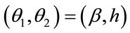 , the scalar-curvature function is computed through the below expression [1-15]:
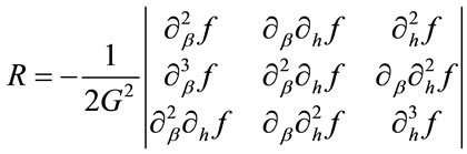 (1)
(1)
where f is the reduced free energy on each site, and  [1-5]. The value of G is defined by the following equation [6-10]:
 (2)
(2)
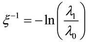
The only quantity defines a high-order transition near the critical point is the correlation length  [11-15]. The scalar curvature according to
  becomes dependent on this quantity in which d is the number of system’s dimensions [16-22]. If it is assumed that the super-scale equation
 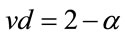 is true, we will have then [2-20]:
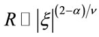 (3)
(3)
A solvable model is considered to study the behavior of R. The one-dimensional Ising model possesses this feature. According to Equation (1), the scalar curvature obtained for this model is as follows [23-25]:
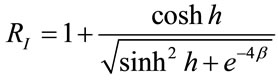 (4)
(4)
In this case,  is a positive value, and becomes divergent only at zero temperature and zero fields (critical point). The correlation length is given by the below equation:
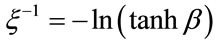 (5)
(5)
Near the critical point, we have ; and in comparison with Equation (3), it is in accordance with
  and
and  that is expected for these exponents.
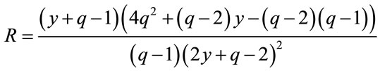
Through Equation (4), the scalar curvature for the onedimensional Potts model is calculated as below [23-25]:
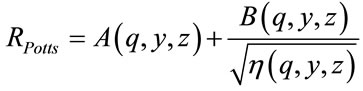 (6)
(6)
where , and
, and . In the above equation, the expressions A and B are as follows:
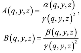 (7)
(7)
In proportion to y and z, these expressions are functions with slow changes, and do not become divergent at the limited temperature and field (physical). The value of  is computed by the below function:
 (8)
(8)
In general, the expressions of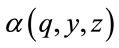 ,
,  , and
, and  are very long for different values of q (however, they are easily achieved).
For , Equation (6) is transformed into the following equation that is Equation (4) for the Ising model:
 (9)
(9)
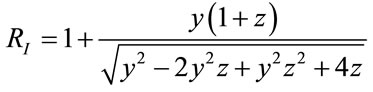
In the zero fields , the expression R for the onedimensional Potts model is acquired as a much more compact form:
 (10)
(10)
It is observed that through changing y from 1 to ∞, the value of R changes from  to ∞. Generally, the geometrical shape of R, that is a function of y and z, is the same. The correlation length for one-dimensional Potts model is defined as same as the correlation length for one-dimensional Ising model:
 (11)
(11)
in which the eigenvalues of transfer matrix of one-dimensional Potts model is as follows:
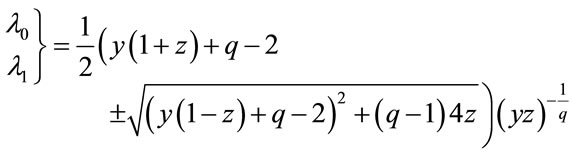 (12)
(12)
For  and
and , we have
 . Therefore, according to
  in
in , the anticipated scaled value of R for one-dimensional Potts model is obtained again. The exponents are also similar to the one-dimensional Ising model (
 ,
, ).
).
In Figure 1, the illustration of function R for Ising model ( ) is depicted. The symmetry
  of Ising model with the transform of
  is evident in the graph of R.
2. Analytical and Numerical Methods
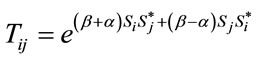
The general Hamiltonian of this model is written as the below form [26-29]:
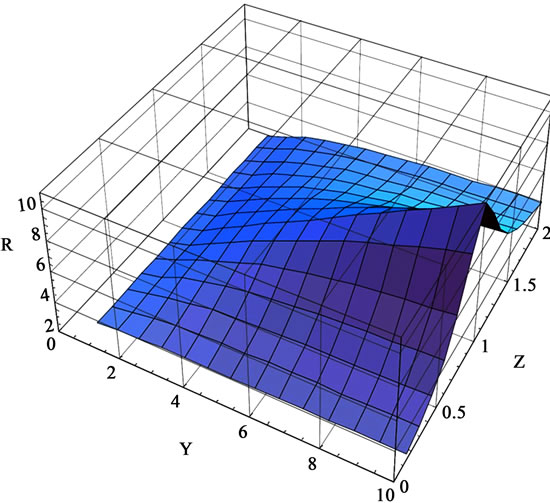
Figure 1. The scalar curvature for the one-dimensional Ising model. The maximum value of R is along the line z = 1.
 (13)
(13)
where ; α and β are two constants. The values of spins are as follows:
 (14)
(14)
In other words, instead of  Ising, spins choose q states. The values of Ising spin are obtained in the particular state of
 . Based on the Perron-Frobenius theorem, the one-dimensional systems do not show phase transition. However, this model does not conform to this theorem on account of being mixed; despite being onedimensional, it has the first-order phase transition [26- 32]. The mixed model has various applications. Such actions in the lattice gauge theories are known as the Chern-Simons action, and effectively substituted for the fermions’ action in the gauge theories [33]. The mixed spin model causes the computations of the two-dimensional gravity and coupling of spins and random surfaces, and the determination of these models’ critical exponents as a solvable theory to improve [26-29]. In these states, first, a chain containing N spins with the periodic boundary condition of
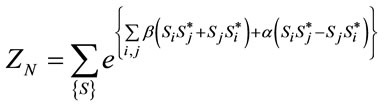
  is considered. The general partition function is written as the following form:
 (15)
(15)
Through considering the nearest neighbors, we have:
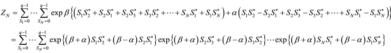 (16)
(16)
Now, each of the above terms can be considered as the transfer matrix’s elements:
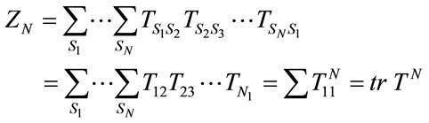 (17)
(17)
in which the general form of the transfer matrix’s elements is as follows:
 (18)
(18)
Since each of  s can have q values, the above matrix is a
  matrix. As an example, this matrix for
  is as follows:
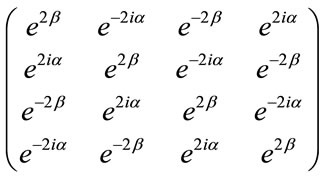 (19)
(19)
This matrix’s eigenvalues are as follows:
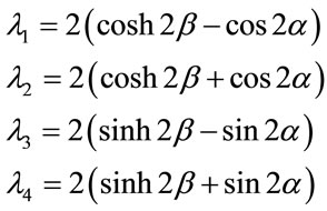 (20)
(20)
Provided the above expressions’ maximum eigenvalue is determined, the reduced free energy on each site can be calculated. For this purpose, the problem is numerically solved. This can be conducted for a value of β, and to change the other parameter (α). Figures 2 and 3 demonstrate the mixed model’s phase transition for the constant values of β. Through studying these curves, and considering the absence of the first-order derivative in where the two peaks separate from the curve, the maximum eigenvalue can be computed. The absence of derivative in these peaks means the first-order phase transition. After the calculation of maximum eigenvalue, the scalar curvature is computed:
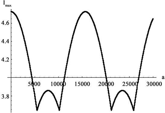
Figure 2. The curve of maximum eigenvalue for the onedimensional mixed lattice for β = 0.415 and q = 4.
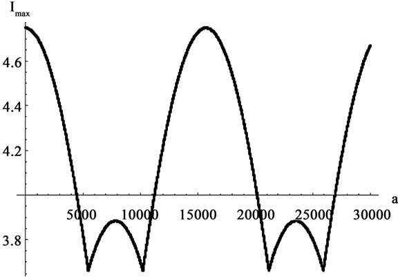
Figure 3. The curve of maximum eigenvalue for the onedimensional mixed lattice for β = 0.43 and q = 4.
 (21)
(21)
3. Results and Discussion
In this paper, the scalar curvature of one-dimensional mixed model for the particular case ( ) is calculated. The importance of this computation is that the scalarcurvature model is applicable not only to the systems with second-order phase transition but also to the systems with first-order phase transition. Hitherto, the systems with first-order phase transition have not been studied using the scalar-curvature model. For the first time, the possibility of applying this model to such problems is mooted in this work. In this regard, it is essential to determine the maximum eigenvalue among the four eigenvalues achieved in the previous section, and in proportion to the variables α and β. After this stage, the free energy is computed according to Equation (22) to determine the value of R. Then, through Equation (4), the scalar curvature is obtained for the four existing eigenvalues. The simplified values of scalar curvature for the four mentioned eigenvalues are as follows:
 (22)
(22)
The scalar curvature for the maximum eigenvalue of transfer matrix is selected among the above four values. This means that changing the values of α and β, the maximum eigenvalue is substituted among the four existing eigenvalues, since the functions constituting these eigenvalues are trigonometric functions. In Figure 4, the three-dimensional graph of maximum eigenvalue is illustrated. On this surface, points’ derived curve is discontinuous for a value of β and along a line of variable α are the system’s transition points being in the surface’s depth in the figure. Figures 5 and 6 indicate the curve of changes in R for different values of β. Through investigating these curves, it can be observed that the value of R becomes divergent (the same as Ising and Potts models) in the points the derived curve has discontinuity (critical point).
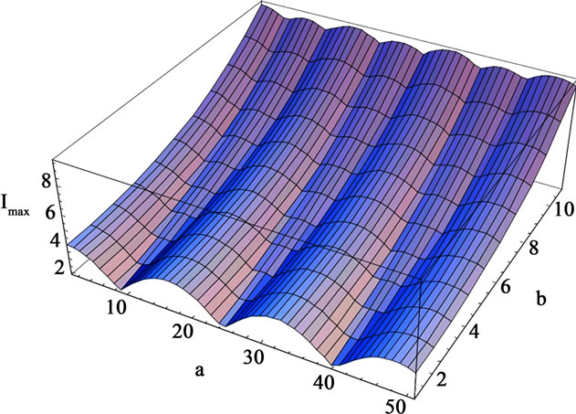
Figure 4. The maximum eigenvalue according to the different values of α and β in the one-dimensional mixed spin model and for q = 4.

Figure 5. The curve of scalar curvature for the one-dimensional mixed lattice for β = 0.415 and q = 4.
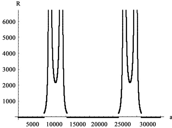
Figure 6. The curve of scalar curvature for the one-dimensional mixed lattice for β = 0.43 and q = 4.
Generally, analytically computing the mixed model’s scalar curvature for every desirable q is difficult in mathematical terms. The numerical methods can be employed to calculate this quantity for every value of q. This can be performed after calculating eigenvalues and free energy’s derivatives in proportion to β and h. Finally, the scalar curvature of R is computed using Equation (1). An interesting event occurs in the computation of R for the three-state model. In this special case, the transfer matrix’s eigenvalues are obtained as follows:
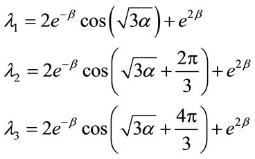 (23)
(23)
Through utilizing these values, and calculating the value of R for each of them, it can be concluded that all the three values of R are equal ( ). The reason why these three values are equal and the phase transition is not shown still remains unknown to us. In this regard, this matter can be studied as another problem.
4. Conclusion
In this paper, through the scalar-curvature model, the fourstate one-dimensional mixed model with the first-order phase transition is investigated. The computed scalar curvature becomes divergent at the points this system has phase transition. This result is consistent with the expected quantity and how it behaves for the other models with the second-order phase transition (the same as three-state Ising and Potts models). The present paper’s results indicate that the scalar-curvature model can have an important role to play in the investigation of all the statistical systems with the phase transition of every order; in other words, it is a new mathematical approach toward such problems. However, the Riemannian Bures metric on the space of (normalized) complex positive matrices is used for parameter estimation of mixed quantum states based on repeated measurements just as the Fisher information in classical statistics. It appears also in the concept of purifications of mixed states in quantum physics. Therefore, and also for mathematical reasons, it is natural to ask for curvature properties of this Riemannian metric. Here we determine its scalar curvature and Ricci tensor and prove a lower bound for the curvature on the submanifold of trace-1 matrices. This bound is achieved for the maximally mixed state, a further hint for the statistical meaning of the scalar curvature.
5. Acknowledgements
The work described in this paper was fully supported by grants from the Institute for Advanced Studies of Iran. The authors would like to express genuinely and sincerely thanks and appreciated and their gratitude to Institute for Advanced Studies of Iran.
REFERENCES
- W. Janke, D. A. Johnston and R. Kenna, “Information Geometry and Phase Transitions,” Physica A: Statistical Mechanics and Its Applications, Vol. 336, No. 1-2, 2004, pp. 181-186. doi:10.1016/j.physa.2004.01.023
- G. Ruppeiner, “Thermodynamics: A Riemannian Geometric Model,” Physical Review A, Vol. 20, No. 4, 1979, pp. 1608-1613. doi:10.1103/PhysRevA.20.1608
- G. Ruppeiner, “Riemannian Geometry in Thermodynamic Fluctuation Theory,” Reviews of Modern Physics, Vol. 67, No. 3, 1995, pp. 605-659. doi:10.1103/RevModPhys.67.605
- G. Ruppeiner, “Thermodynamic Curvature and Phase Transitions in Kerr-Newman Black Holes,” Physical Review D, Vol. 78, 2008, pp. 024016-024028.
- G. Ruppeiner, “New Thermodynamic Fluctuation Theory Using Path Integrals,” Physical Review A, Vol. 27, No. 2, 1983, pp. 1116-1133. doi:10.1103/PhysRevA.27.1116
- G. Ruppeiner, “Application of Riemannian Geometry to the Thermodynamics of a Simple Fluctuating Magnetic System,” Physical Review A, Vol. 24, No. 1, 1981, pp. 488-492. doi:10.1103/PhysRevA.24.488
- G. Ruppeiner and C. Davis, “Thermodynamic Curvature of the Multicomponent Ideal Gas,” Physical Review A, Vol. 41, No. 4, 1990, pp. 2200-2202. doi:10.1103/PhysRevA.41.2200
- G. Ruppeiner, “Stability and Fluctuations in Black Hole Thermodynamics,” Physical Review D, Vol. 75, No. 2, 2007, pp. 024037-024047. doi:10.1103/PhysRevD.75.024037
- G. Ruppeiner, “Riemannian Geometric Theory of Critical Phenomena,” Physical Review A, Vol. 44, No. 6, 1991, pp. 3583-3595. doi:10.1103/PhysRevA.44.3583
- G. Ruppeiner, “Comment on Length and Curvature in the Geometry of Thermodynamics,’’ Physical Review A, Vol. 32, No. 5, 1985, pp. 3141-3141. doi:10.1103/PhysRevA.32.3141
- G. Ruppeiner, “Riemannian Geometric Approach to Critical Points: General Theory,” Physical Review E, Vol. 57, No. 5, 1998, pp. 5135-5145. doi:10.1103/PhysRevE.57.5135
- G. Ruppeiner, “Thermodynamics near the Correlation Volume,” Physical Review A, Vol. 31, No. 4, 1985, pp. 2688-2690. doi:10.1103/PhysRevA.31.2688
- G. Ruppeiner, “Riemannian Geometry of Thermodynamics and Systems with Repulsive Power-Law Interactions,” Physical Review E, Vol. 72, No. 1, 2005, pp. 016120- 016133. doi:10.1103/PhysRevE.72.016120
- G. Ruppeiner, “Asymmetric Free Energy from Riemannian Geometry,” Physical Review E, Vol. 47, No. 2, 1993, pp. 934-938. doi:10.1103/PhysRevE.47.934
- G. Ruppeiner, “Thermodynamics at Less than the Correlation Volume,” Physical Review A, Vol. 34, No. 5, 1986, pp. 4316-4324. doi:10.1103/PhysRevA.34.4316
- H. Janyszek and R. Mrugała, “Riemannian Geometry and the Thermodynamics of Model Magnetic Systems,” Physical Review A, Vol. 39, No. 12, 1989, pp. 6515-6523. doi:10.1103/PhysRevA.39.6515
- H. Janyszek and R. Mrugała, “Geometrical Structure of the State Space in Classical Statistical and Phenomenological Thermodynamics,” Reports on Mathematical Physics, Vol. 27, No. 2, 1989, pp. 145-159. doi:10.1016/0034-4877(89)90001-3
- H. Janyszek, “On the Riemannian Metrical Structure in the Classical Statistical Equilibrium Thermodynamics,” Reports on Mathematical Physics, Vol. 24, No. 1, 1986, pp. 1-10. doi:10.1016/0034-4877(86)90036-4
- H. Janyszek, “On the Geometrical Structure of the Generalized Quantum Gibbs States,” Reports on Mathematical Physics, Vol. 24, No. 1, 1986, pp. 11-19. doi:10.1016/0034-4877(86)90037-6
- H. Janyszek, “On the Connection between the Classical Spin and the Lorentz Group,” Reports on Mathematical Physics, Vol. 13, No. 3, 1978, pp. 311-313. doi:10.1016/0034-4877(78)90058-7
- D. C. Brody and A. Ritz, “Information Geometry of Finite Ising Models,” Journal of Geometry and Physics, Vol. 47, No. 2-3, 2003, pp. 207-220. doi:10.1016/S0393-0440(02)00190-0
- D. C. Brody and L. P. Hughston, “Geometric Quantum Mechanics,” Journal of Geometry and Physics, Vol. 38, No. 1, 2001, pp. 19-53. doi:10.1016/S0393-0440(00)00052-8
- B. P. Dolan, D. A. Johnston and R. Kenna, “The Information Geometry of the One-Dimensional Potts Model,” Journal of Physics A: Mathematical and General, Vol. 35, No. 43, 2002, p. 9025. doi:10.1088/0305-4470/35/43/303
- B. P. Dolan, W. Janke, D. A. Johnston and M. Stathakopoulos, “Thin Fisher Zeros,” Journal of Physics A: Mathematical and General, Vol. 34, No. 32, 2001, p. 6211. doi:10.1088/0305-4470/34/32/301.
- W. Janke, D. A. Johnston and R. Kenna, “GeometroThermodynamics of the Kehagias-Sfetsos Black Hole,” Journal of Physics A: Mathematical and Theoretical, Vol. 43, No. 42, 2010, p. 425206. doi:10.1088/1751-8113/43/42/425206.
- J. F. Wheater and J. Correia, “The Spectral Dimension of Non-Generic Branched Polymers,” Nuclear Physics B— Proceedings Supplements, Vol. 73, No. 1-3, 1999, pp. 783-785. doi:10.1016/S0920-5632(99)85202-5
- J. Correia and J. F. Wheater, “Three-State Complex Valued Spins Coupled to Binary Branched Polymers in TwoDimensional Quantum Gravity,” Nuclear Physics B— Proceedings Supplements, Vol. 63, No. 1-3, 1998, pp. 754-756. doi:10.1016/S0920-5632(97)00894-3
- J. Correia and J. F. Wheater, “A Simple Model of Dimensional Collapse,” Physics Letters B, Vol. 388, No. 4, 1996, pp. 707-712. doi:10.1016/S0370-2693(96)01223-3
- J. Correia and J. F. Wheater, “The Spectral Dimension of Non-Generic Branched Polymer Ensembles,” Physics Letters B, Vol. 422, No. 1-4, 1998, pp. 76-81. doi:10.1016/S0370-2693(98)00055-0
- J. A. Cuesta and A. Sánchez, “General Non-Existence Theorem for Phase Transitions in One-Dimensional Systems with Short Range Interactions, and Physical Examples of Such Transitions,” Journal of Statistical Physics, Vol. 115, No. 3-4, 2004, pp. 869-893. doi:10.1023/B:JOSS.0000022373.63640.4e
- J. A. Cuesta, A. Sánchez and F Dominguez-Adame, “Self-Consistent Analysis of Electric Field Effects on Si Delta-Doped GaAs,” Semiconductor Science and Technology, Vol. 10, No. 10, 1995, p. 1303. doi:10.1088/0268-1242/10/10/002.
- J. A. Cuesta and A. Sánchez, “A Theorem on the Absence of Phase Transitions in One-Dimensional Growth Models with On-Site Periodic Potentials,” Journal of Physics A: Mathematical and General, Vol. 35, No. 10, 2002, p. 2373. doi:10.1088/0305-4470/35/10/303.
- T. G. Kovacs and J. F. Wheater, “The Phase Structure of Two-Dimensional Pure Lattice Gauge Theories with Chern Term,” Modern Physics Letters A, Vol. 6, No. 30, 1991, pp. 2827-2835.
NOTES
*Corresponding author.