Applied Mathematics
Vol.07 No.16(2016), Article ID:71469,28 pages
10.4236/am.2016.716160
On Applications of Generalized Functions in the Discontinuous Beam Bending Differential Equations
Dimplekumar Chalishajar, Austin States, Brad Lipscomb
Department of Applied Mathematics, Virginia Military Institute (VMI), Lexington, USA

Copyright © 2016 by authors and Scientific Research Publishing Inc.
This work is licensed under the Creative Commons Attribution International License (CC BY 4.0).
http://creativecommons.org/licenses/by/4.0/


Received: June 24, 2016; Accepted: October 22, 2016; Published: October 25, 2016
ABSTRACT
This paper discusses the mathematical modeling for the mechanics of solid using the distribution theory of Schwartz to the beam bending differential Equations. This problem is solved by the use of generalized functions, among which is the well known Dirac delta function. The governing differential Equation is Euler-Bernoulli beams with jump discontinuities on displacements and rotations. Also, the governing differential Equations of a Timoshenko beam with jump discontinuities in slope, deflection, flexural stiffness, and shear stiffness are obtained in the space of generalized functions. The operator of one of the governing differential Equations changes so that for both Equations the Dirac Delta function and its first distributional derivative appear in the new force terms as we present the same in a Euler-Bernoulli beam. Examples are provided to illustrate the abstract theory. This research is useful to Mechanical Engineering, Ocean Engineering, Civil Engineering, and Aerospace Engineering.
Keywords:
Mechanics of Solids, Discontinuities in a Beam Bending Differential Equations, Generalized Functions, Jump Discontinuities

1. Introduction
This article introduces the method for computing lateral deflections of plane beams undergoing symmetric bending. Reviewers should be acquainted with: integration of ordinary differential Equations, and statics of plane beams under symmetric bending.
Our primary objective is to apply the discontinuous beam bending differential Equation to different application obviously representing beam bending. One of the most common types of structural components is a beam, recommended more in Civil and Mechanical Engineering. A beam resembles as a bar-like structural that is used to support transverse loading and carry it to the supports. Beams resist against transverse loads through a bending action, which creates compressive longitudinal stresses on one side of a beam and tensile stress on the other side. With these two combinations between compressive longitudinal stress and tensile stress, an internal bending moment starts to occur. In the case of a discontinuous load, we begin applying beam-bending differential Equation for each part of the beam.
All models use some sort of approximation to the underlying physics because beams are three-dimensional bodies.
Transverse loading being resisted on a preferred longitudinal plane is known as a
plane beam. Because the classical beam theory is the simplest and most associated
model for plane beams, it presents assumptions such as:
1) Planar symmetry: The longitudinal axis appears to be straight with a cross section of the beam being longitudinal plane of symmetry. Each sections that lie on the plane, both resultant of the transverse loads. The resultant of the transverse loads acting on each section lies on the plane.
2) Cross sectional variation: The cross section remains constant or varies.
3) Normality: The plane sections are originally normal to the longitudinal axis of the beam remain plane and normal to the reformed longitudinal axis upon bending.
4) Strain energy: Transverse shear and axial forces are ignored, while only internal strain energy from another object accounts for the bending moment deformations.
5) Linearization: The infinitesimal deformation of the beam is brought into the mix due to the consideration of transverse deflections, rotations and deformations.
6) Material model: The heterogeneous beams are fabricated with several elastic and isotropic materials, such as reinforced concrete.
Transverse shear and axial force are ignored, while only internal strain energy from another object accounts for the bending moment deformations. The assumption of infinitesimal deformation is brought into the mix due to the consideration of transverse deflections, rotations and deformations. The assumption is made that heterogeneous beams are fabricated with several elastic and isotropic materials.
Now we will begin our discussion on classical beam theory, also known as The Euler- Bernoulli Beam Theory.
・ Beam coordinates system:
The coordinate system throughout the beam undergoes a transverse loading at a point on the top surface will shorten. As for the other, it will elongate. This causes a neutral surface between the top and the bottom.
・ Beam motion:
We associate beam motion as the loading on a x, y plane beam is structured in to two dimensional displacement field  and
and  u and v are respected as the axial and transverse displacement components with respect to a beam point.
・ Beam loading:
 is denoted as the transverse force per unit length occurs on the plane beam in a positive y direction. We can determine the strong and the weak loading points based on what beam is being used. For instance, support on a simply supported beam is found on the end points that prohibit transverse displacements. In contrast, one side of a cantilever beam does not have an end support, resulting with one being clamped on and the other being free. Airplane wings, diving boards, and stabilizers are prime examples of cantilever beams.
2. Singular Loading Conditions
This section will explain the equivalent distributed force for a family of singular loading condition by using Schwartz’s distribution theory.
Definition 1. Let  be a distributed force. The nth order moment of
  that
that  is given by
 (1)
(1)
Definition 2. Let  be a distributed force in the small open segment (interval).
  Also consider
 (2)
(2)
Then
 (3)
(3)
In 1959, Timoshenko and Woinowsky-Krieger [1] studied the concentrated double moment of the beam, which is the limiting situation of two opposite movements acting on two different separated points. They proved the result in a deflection with a discontinuous slope at the point of the concentrated double movement.
In this article, we want to study the equivalent distributed force in the loading function of a point moment of order n by using the distribution theory, refer [2] . We will show that the loading function for this loading condition is expressed by
 (4)
(4)
where  is the value of double movement and
  is the second distributional derivative of
 .
.
Theorem 1. The equivalent distributed force of a unit moment of order n applied at  is
is
 (5)
(5)
where  is the nth distributional derivative of the Dirac Delta function.
Corollary 1. The equivalent distributed force for an upward concentrated force of magnitude p is
 (6)
(6)
This was obtained by Timoshenko (1976) [3] and Shames (1989) [4] , where the limiting case of a load distributed over a very short portion of a beam. The shearing forces of an Euler-Bernoulli beam can be applied to act as another proof of this representation by using the discontinuity of a concentrated force, appears in Section 3.4.
Corollary 2. The equivalent distributed force of a clockwise concentrated moment of magnitude M is
 (7)
(7)
This result was founded by Shames in (1989) [4] , in which this loading is considered to be the limiting case of two concentrated forces ,
,  apart, when
  goes to zero. The bending moment of an Bernoulli beam can be applied to act as another proof of this representation by using the discontinuity a concentrated moment introduces. It appears in Section 3.3.
Corollary 3. The equivalent distributed force of a concentrated double moment is given by Equation (4). As Timoshenko and Woinowsky-Krieger (1959) [1] mention, this loading results in a deflection with a discontinuous slope at the point of double moment. We see later that, in an Euler-Bernoulli beam with a jump discontinuity in slope, this forcing function appears.
3. A Mathematical Explanation for Corner Condition in Classical Plate Theory and Equally Distributed Force for Distributed Moments
In this section we obtain the equivalent distributed force of a distributed moment. We then give a mathematical explanation for corner condition in classical plate theory.
It can be shown that the force function of a distributed moment,  , can be expressed in terms of m and
 (8)
(8)
But distribution theory shows that for any function f
 (9)
(9)
Hence,
 (10)
(10)
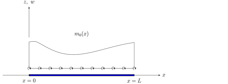
Accordingly, for a distributed moment the first distributional derivative of , is the forcing function. Imagine a beam that has a length of L under a distributed moment
 , (see Figure 1(a)). The moment can be written as
 (11)
(11)
Hence,
 (a)
(a)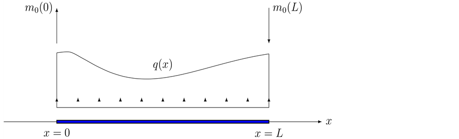 (b)
(b)
Figure 1. (a) A beam under a distributed moment. (b) The equivalent force system.
 (12)
(12)
where H is Heaviside’s function. When substituting Equation (12) into Equation (10), the output is
 (13)
(13)
The distributed moment is equivalent to the distributed force  on both end points of the beam given by
 . Also distributed moment is equivalent to two
concentrated forces  and
and  at
at  and
and , respectively, as shown in Figure 1(b). Similarly, if
  is a partially distributed moment in
  is equivalent to a distributed force in this interval
  and two concentrated forces at
  and
and .
.
 (14)
(14)
Corner condition: Timoshenko and Woinowky-Krieger (1959) [1] were unable to explain the corner condition mathematically, although they mentioned it physically as below:
・ Corner conditions definition―physically: The polygonal loaded plates will usually produce concentrated reaction at corner points with the distributed reaction along the edges.
・ Corner conditions definition―mathematically: In classical plate theory  Equation (14) consists of a system of distributed forces and two concentrated forces as the corner points.
Note: Corner conditions phenomenon does not appear in sheer deformation theo- ries.
4. Representing Point Loads and Moments through Jump Discontinuities, Deflection, and Flexural Stiffness Using the Euler-Bernoulli Beam Theory
The classical method of solving the differential Equation of Euler-Bernoulli beam with jump discontinuity in slope, deflection and flexural stiffness, is to solve the problem on both sides of the discontinuities and then apply boundary and continuity conditions. Here we will solve a problem of differential Equation in the space of generalized functions we solve the problem as a single beam using generalized functions therefore we will consider only one point of jump discontinuity and then generalize this idea with n singular points of an Euler-Bernoulli beam.
Euler-Bernoulli beam theory provides the following displacement field assumptions:


 (15)
(15)
where ,
,  ,
,  are displacement components along the x, y, and z axes respectively. The beam lies along the x-axis and the loads are applied vertically along the z-axis. We can use Equation (15) and the foundation of virtual work, the governing equilibrium Equation can be declared as:


 (16)
(16)
where EI is the flexural stiffness and q is a distributed force and is called the loading function.
The first three derivatives of w are continuous and the fourth derivative is piecewise continuous, only when q is a piecewise continuous function. On the other hand, there are some equivalent distributed conditions for which the loading function cannot be declared as a classical function. A general case of these conditions were studied in Section 2. However, displacement of the beam or its derivatives can sometimes have discontinuities that are separate from the loading condition. That introduces the focus of this section.
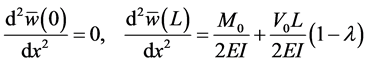
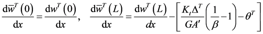
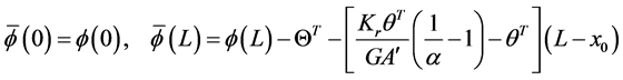
The beam shown in Figure 2 is of length L and the boundary conditions are arbitrary at . The flexural stiffness of the beam is changed periodically at
 . This point will also house discontinuities in slope and deflection. The most general case uses a combination of an internal hinge with a rotational spring along with a shear-free connection with a translational spring. The constants of the rotational and translation springs are
  and
and , respectively. Now we take
 (17)
(17)
 (18)
(18)
The beam has two components to it, segments AB and BC. Hence, why the Heaviside’s function is applied.
 (19)
(19)
where w is the deflection of the beam,  is the deflection of the segment AB, and
  is the deflection of the segment BC. After the calculation given in the appendix, the governing differential Equation of the beam is

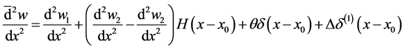

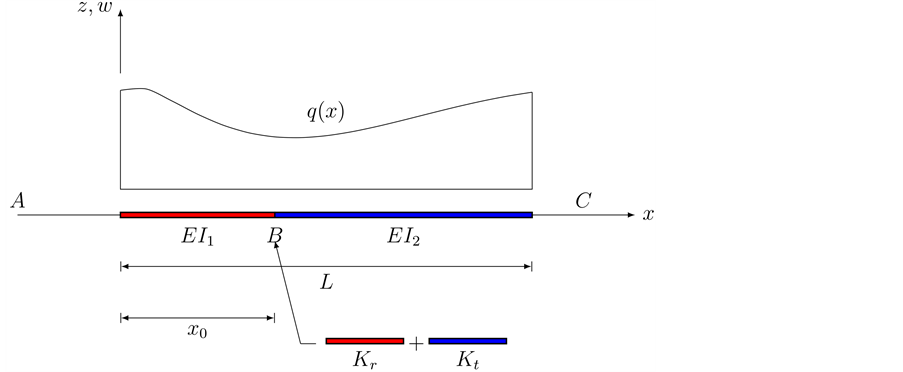
Figure 2. A beam with a jump discontinuity in slope, deflection, and flexural stiffness with arbitrary boundary conditions under a distributed force.
 (20)
(20)
where the distributional differentiation is denoted by the bar. As can be seen having jump discontinuities in slope and deflection is equivalent to having double and triple point moments ,
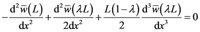
,  at the point of jump discontinuities. Also, continuity conditions can be written as
 (21)
(21)
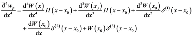
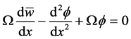
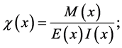
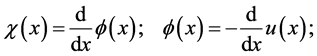
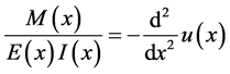
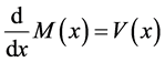
when you apply the four boundary conditions at  as well as the continuity conditions from Equation (21), you are able to gather the deflection w. As can be seen only the force term changes; the form of the operator of the differential Equation is the same as that of Equation (16).
4.1. Solution Procedure
Kanwal [5] proposed a method, that we are about to use, in order to solve a differential Equation in the space of a generalized function. The general solution is
 (22)
(22)
 and
and  are solutions to the following differential Equations
 (23)
(23)
 (24)
(24)
when finding , we assume that
 (25)
(25)
Hence,
 (26)
(26)
Equating the coefficient of the generalized functions in Equation (24) and Equation (26), we are able to obtain
 (27)
(27)
 (28)
(28)
 (29)
(29)
After solving Equation (27) and applying the initial conditions (29), we are able to obtain
 (30)
(30)
Solving Equation (23) for , we have four integration constants. Applying the four boundary conditions at
  for
for  and the continuity conditions (21), we obtain the beam deflection. Obviously, this is not an efficient method and has no superiority over the classical method. A more efficient method is proposed here for calculating the beam deflection.
4.2. Auxiliary Beam Method
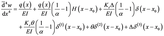
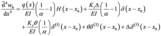
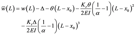
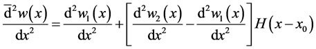
Suppose w represents the deflection of an Euler-Bernoulli beam with jump discontinuities in slope, deflection, and flexural stiffness at the point . The deflection is defined as:
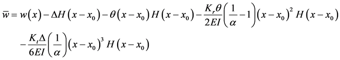 (31)
(31)
 is the classical function. Using Equation (31) in Equation (20) allows us to obtain
 (32)
(32)
We also have, from Equation (31)

 (33)
(33)

 (34)
(34)

 (35)
(35)
The continuity conditions for the auxiliary beam are:
 (36)
(36)
Therefore, instead of solving two differential Equations for the two beam segments and applying eight boundary and continuity conditions, only one differential Equation with six boundary and continuity Equations is solved. To clarify the method, three examples are solved in the next section.
Three examples are presented and solved in order to show the efficiency of The Euler-Bernoulli Beam Theory with jump discontinuities.
Example 1. This is an example of a internal hinged beam under a uniform distributed force. The beam shown in Figure 3 is clamped at  and simply supported at
 .
.
The flexural stiffness is constant.
 (37)
(37)
From Equation (32), the G.D.E of the auxiliary beam is
 (38)
(38)
 (39)
(39)
 (40)
(40)
 (41)
(41)
Lastly,
 (42)
(42)
It is known that for this beam,
 (43)
(43)
Using Equation (33) through Equation (35) we are able to find,
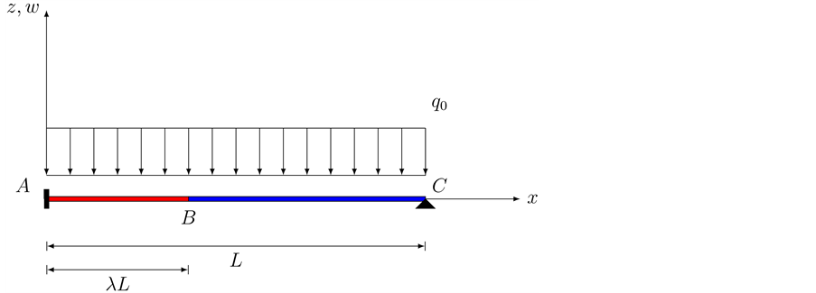
Figure 3. A clamped, simply supported beama with an internal hinge under a uniform distri- buted force.
 (44)
(44)
Using Equation (27) and Equation (29) we are able to obtain  and
and 
 (45)
(45)
Now, using Equation (42) and Equation (44) we obtain
 (46)
(46)
We also find that
 (47)
(47)
Therefore, from Equation (31) we can derive
 (48)
(48)
Example 2.
This example uses a beam that has a jump discontinuity at , shown in Figure 4.
For this beam we know,
 (49)
(49)
Using Equation (49) we can find the G.D.E of the auxiliary beam
 (50)
(50)
 (51)
(51)
 (52)
(52)
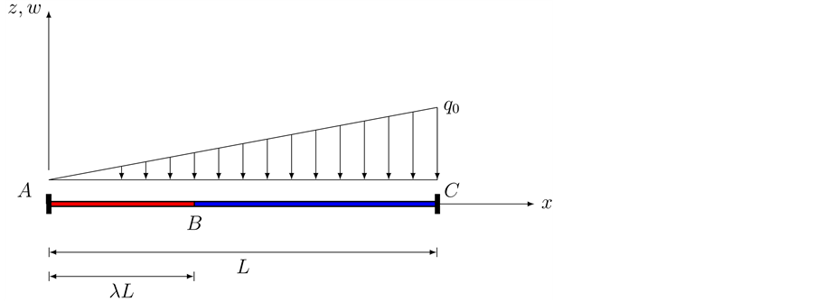
Figure 4. A double clamped beam with an internal shear-free connection under a linearly vary- ing distributed force.
 (53)
(53)
Thus,
 (54)
(54)
We know the following is true for this beam,
 (55)
(55)
 (56)
(56)
Now, using Equation (33) through Equation (35) we have
 (57)
(57)
 (58)
(58)
Now using Equation (54), Equation (57) and Equation (58), we obtain


In a similar way as Example 1, we can find  to be
to be
 (59)
(59)
 (60)
(60)
Now, from Equation (31)
 (61)
(61)
Example 3. A Simply supported beam under a uniform distributed force with jump discontinuity in flexural stiffness at  is shown in Figure 5.
For this beam
 (62)
(62)
and the deflection of the beam is defined as:
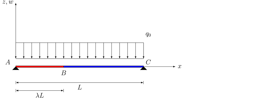
Figure 5. A simply supported beam with a jump discontinuity in flexual stiffness under a uniform distributed force.
 (63)
(63)
The governing differential Equation of the beam is
 (64)
(64)
The boundary and continuity conditions are
 (65)
(65)
 (66)
(66)
 (67)
(67)
When you combine the boundary and continuity Equations, you will get
 (68)
(68)
 (69)
(69)
 (70)
(70)
From Equation (54) we are able to obtain,
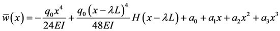 (71)
(71)
When applying the boundary and continuity conditions to Equation (61), we are able to obtain
 (72)
(72)
From Equation (57) we are able to obtain,
 (73)
(73)
Therefore, from Equation (64) we obtain
 (74)
(74)
Assuming  gives us the deflection of a simply-supported beam with a constant flexural stiffness EI under a uniform distributed force
 (75)
(75)
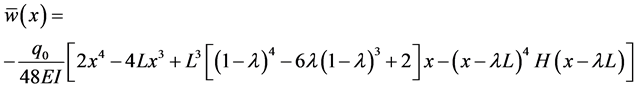
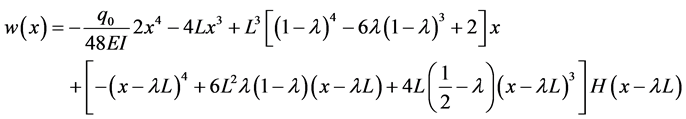
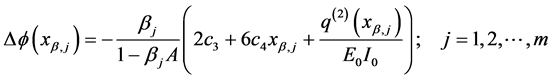
For n point loads (moment or force) one has to use  differential Equation and has to apply
  boundary and continuity conditions. By using Macauly’s bracket we have only one expression for the bend moment and loading function using the singularity function matter. In this case only one differential Equation with four boundary conditions are required to be solved.
In the case of n jump discontinuities, if one uses the auxiliary beam methods, shown in this article, instead of solving  differential Equations and applying
  boundary and continuity conditions need to be solved. In almost all practical problems, we do not have all three kinds of discontinuities at the same point (ie if a beam has n internal hinges, then the number of continuity Equations is reduced to n).
In Section 3 for finding the governing differential Equation of an Euler-Bernoulli beam with jump discontinuities, the beam was partitioned to continuous beam segments. The next section will use the same ideas in order to find the equivalent distributed forces for point forces and point moments.
4.3. Equivalent Force Function for Concentrated Force and Moment: A Nonclasical Approach
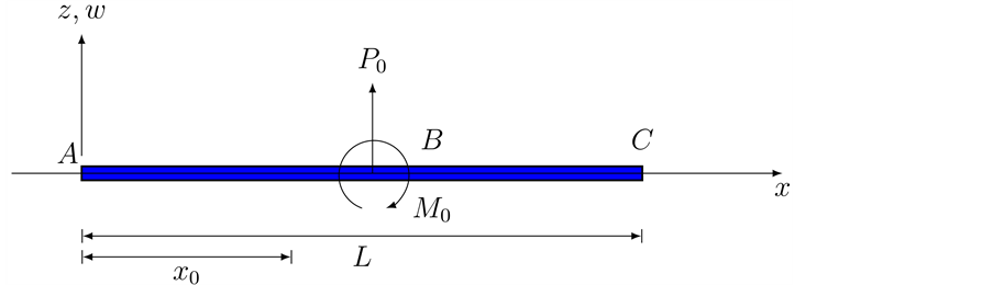
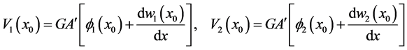
Here we will use that a concentrated force and a concerntrated moment represnt jump discontinities into shearing orce (the third derivative of the beam deflection) and the bending moment (the second derivative of the beam deflection) respectively, of an Euler-Bernoullie beam. As mentioned earlier, in Section 2, the classical proof of Equation (6) and Equation (7) is based on considering the singular loading condition as a distributed force over a very short length of the beam. The concentrated force and the concentrated moment introduced jump discontinuities into the sheering force, third derivative of the Equation, and the bending moment, second derivative of the Equation, of an Euler-Bernoulli beam. In this section we will study a non classical approach for a concentrated force of magnitude P, Equation (6) and a concentrated moment of M Equation (7). Figure 6 shows a beam with a concentrated force  and a concentrated moment
  applied at
 . The beam AC may be assumed to be composed of two beam segments, AB and BC. The deflections of the two beam segments AB and BC are denoted by w1 and w2 respectively. There is no loading for
  and
and ; hence, we have
 (76)
(76)
 (77)
(77)
w is the deflection of the beam and can be written as
 (78)
(78)
We know that the magnitudes of  and
and  are equal at
 , the same is true for their first derivatives. Therefore,
 (79)
(79)
From the figure above, we can write

 (80)
(80)
Then,
 (a)
(a)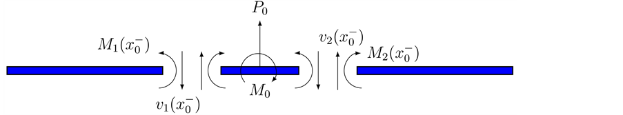 (b)
(b)
Figure 6. (a) A beam under a concentrated force and a concentrated moment. (b) Moment and shear discontinuity at the point of the action of concentrated loads.

 (81)
(81)
If you differentiate both sides from Equation (82) with respect to x, you get
 (82)
(82)
also
 (83)
(83)
Now, from Equation (76), Equation (77) and Equation (86) we obtain
 (84)
(84)
Therefore, the equivalent force function is
 (85)
(85)
5. Timoshenko Beam with Jump Discontinuities
Much like the work introduced on Euler-Bernoulli beams; we can also acquire jump discontinuities in slope, deflection, flexural stiffness, and shear stiffness to a system of differential Equations of a Timoshenko beam [6] . Differentiation between Euler- Bernoulli beams and Timoshenko beams are the distant shear deformation in the Timoshenko beams. Shear deformation is where a force is being applied on one part and another force is being applied on another part, but in the opposite direction. Along the x, y, and z-axes, are displacement components ,
,  , and
, and . The displacement field is provided by the Equations


 (86)
(86)
 ,
,  , and
, and  are displacement components in the
  plane. Also,
  is the rotation of the Timoshenko beam about the y-axis and the superscript T shows the deflection of the Timoshenko beam. The Governing system of differential Equations can be written as,

 (87)
(87)
the shear modulus, G, is a distinguished ratio of the shear stress over the shear strain. The shear stress is the force applied to a certain amount of area it is applied to. The shear strain on the other hand, is the rate of change in displacement of the strain combine with ,
,
 (88)
(88)
the ratio of shear and flexural stiffness has now been defined.
We can substitute Equation (88) into Equation (87) yields,

 (89)
(89)
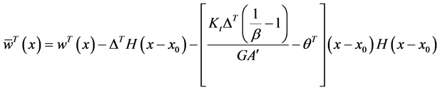
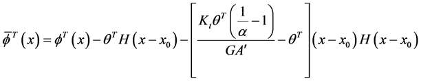
Next, ponder a Timoshenko beam has jump discontinuities in the slope, deflection, shear stiffness, and flexural stiffness at  on its length L. We refer to the heavy- side function as used for the Euler-Bernoulli beam to initiate the two Equations of deflection and rotation of the Timoshenko beam, we can write

 (90)
(90)
Because deflection and rotation both have jump discontinuities at , we write
 (91)
(91)
It is known that
 (92)
(92)
and
 (93)
(93)
Also, for an infinitesimal element including the discontinuity point at equilibrium implies

 (94)
(94)
As we can see from Equation (94),  and
and  are the stiffness of the translational and rotational springs at
 . So after reviewing and comparing Equation (92), Equation (93) and Equation (94),

 (95)
(95)
where

 (96)
(96)
Differentiating Equation (90), we obtain
 (97)
(97)
 (98)
(98)
and
 (99)
(99)
 (100)
(100)
The deflection and rotation of each beam segment have continuous derivatives and hence they are governed by Equation (84), thus
 (101)
(101)
 (102)
(102)
and
 (103)
(103)
 (104)
(104)
Now if we let  and
and  we can obtain the governing system of equi-
librium Equations for the beam from Equation (97) through Equation (104),
 (105)
(105)
5.1. Auxiliary Beam Method
This section shows the similarities between the Euler-Bernoulli method and the Timoshenko methods by providing a Timoshenko method example. You can compare it to the Euler-Bernoulli method from earlier. The auxiliary beam is defined for a Timoshenko beam with internal jump discontinuities. The deflection and rotation of the beam are defined below:
 (106)
(106)
Substitution Equation (106) into Equation (105) yields,

 (107)
(107)
The boundary conditions for this beam can be found by using the relations shown below:
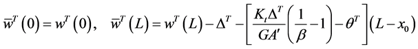
 (108)
(108)
and
 (109)
(109)
The continuity condition may be expressed as
 (110)
(110)
The next section will provide an example to clarify the method shown.
5.2. Timoshenko Beam Example
Suppose the beam used in Example 1 is now a Timoshenko beam, from Equation (107) and Equation (37) we obtain,
 (111)
(111)
 (112)
(112)
The boundary and continuity conditions for this beam can be written as,

 (113)
(113)
After solving this system and applying the boundary and continuity conditions we obtain
 (114)
(114)
 (115)
(115)
 (116)
(116)
From Equation (106) we obtain
 (117)
(117)
 (118)
(118)
Hence,
 (119)
(119)
 (120)
(120)
As the shear stiffness approaches infinity the effect of shear deformation diminishes until it disappears entirely. From Equation (47) and Equation (116), it is seen that
 (121)
(121)
6. Dirac-Delta Function in the Static Analysis of Multi-Cracked Euler-Bernoulli Beams
Structural analysis of multi-cracked beams is of greater engineering interest. Research in this area has been mainly concentrated on two classes of problems:
・ definition of appropriate linear and non-linear models for representing the effects of cracks under static and dynamical loadings and
・ detection of position and severity of the damage by using either static or dynamic tests.
Here we will study an effective and physically based linear modeling of multi-cracked beams subject to the static loading. This result is useful for treating any type of concentrated damage occurring in slender and short beams, e.g. corrosion of steel bars in reinforced concrete members, defects of material and attacks of biotic agents in timber elements etc.
The idea of treating multi-cracked beams with equivalent linear springs at the crack’s position is based on the portion of each member into undamaged pieces between two consecutive cracks. For slender Euler-Bernoulli beam, the governing 4th order differential Equation of bending can be written for each subsystem, but it is necessary to impose the pertinent continuity conditions between adjacent subsystems to obtain the static response of the whole beam.
As a result, the computational effort increases with the number of cracks, i.e for n cracks along the beam,  algebraic Equations have to be solved to compute
  integration constants. But this method is inefficient for identifications purposes, when analysis are repeated until position and severity of the damage are found. So one can use finite element method (FEM) in which stiffness matrix and load vector of the non-cracked Euler-Bernoulli beam are modified with some dimensionless coefficients with effects of internal cracks.
Here we will be using generalized functions to handle static and kinematical discontinuities along the beam. Here we require the enforcement of continuity conditions at each jump, and hence additional integration constants are needed. This issue can be tracked in the formulation of “rigidity modeling”, which consists of singularities in the flectual stiffness represented by Dirac’s delta functions, which in turn are equivalent to internal hinges with rotational linear-elastic springs.
In this work, a non-trivial generalization to multiple discontinuities in the curvature and the slope functions of the integration procedure is presented. The case of Euler-Bernoulli beams under static loads is treated; discontinuities in the curvature and the slope function are modeled as unit step distributions and Dirac’s delta, respectively, in the flectural stiffness of the beam. Moreover, the presented procedure is also extended to cases of discontinuities in the axial displacement and in the vertical deflection modeled as Dirac’s deltas in the axial stiffness and the shear stiffness, respectively.
6.1. Solution of Euler-Bernoulli Beam with a Flectural Stiffness Model with Multiple Singularities
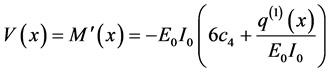
The well known static governing Equations of Euler-Bernoulli beam with variable Young modulus  and moment of inertia
  are given by
 (122)
(122)
 (123)
(123)
 (124)
(124)
where  is the external load,
  and
and  are the shear force and the bonding moment, respectively,
  ,
,  , and
, and  are the deflection, slopes and curvature functions, respectively, and prime denotes differentiation where the spatial coordinate x spanning from 0 to the length L of the beam. Since Equation (124),
 (125)
(125)
By Equation (123),
 (126)
(126)
Also, from Equation (123),
 (127)
(127)
and by Equation (122) we get,
 (128)
(128)
By combining Equation (127) and Equation (128), we get

 (129)
(129)
The flexural stiffness model with a single singularity described by means of a suitable distribution as follows:
 (130)
(130)
The same model is reconsidered and extended to the case of multiple singularities.
Equation (130) describes a constant flexural stiffness  with n-variations of intensity
  and abscissas
 , modeled by means of n distributions here indicates as
 . Two types of distribution, such as unit step distribution
  and Dirac’s delta
  are considered in Equation (130) for the Euler-Bernoulli beam, which leads to two different models as follows

 (131)
(131)
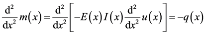
The flexural stiffness provided by Equation (131) describes a beam showing concentrated jumps in the Young modulus  and the inertia moment
  of the cross section (Figure 7). In this case, for the flexural stiffness
  to be non-negative, the only constraints to be imposed on jump intensities
  for the model described by Equation (131) are
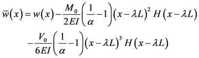
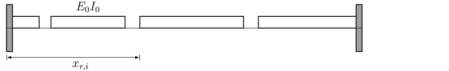
 . On the other hand, if the flexural stiffness is given by Equation (131) for the case of a single Dirac’s delta, the slope function will show n concentrated jumps induced by the presence of internal hinges endowed with rotational springs, as depicted in (Figure 8(a)). For this case, constraints on
  will be discussed later.
Now we will study two different flexural stiffness models given by Equation (131) using the theory of distributions. Further, we present the model with the presence of two different singularities.
6.2. Solution of Euler-Bernoulli Beams in Presence of Multiple Curvature Discontinuities
Here we study the case of multiple jump discontinuities in the flexural stiffness, provided by Equation (131). Such case has been discussed for single (Yavari et al., 2000) [7] and double jumps (Yavari and Sarkani, 2001) [8] . But in those procedures enforcement of continuity conditions (where jumps appear) is required. We provide closed form solution for any number and position of the discontinuities.
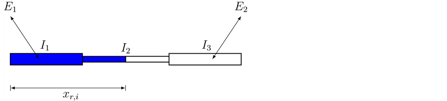
Figure 7. Beam with discontinuities in the Young modulus  and in the moment of inertia
 .
.
 (a)
(a)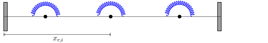 (b)
(b)
Figure 8. (a) A beam with Dirac’s delta singularities in the flexural stiffness which corrosponds to Figure 8(b). (b) A beam with internal hinges and rotational springs with stiffness .
.
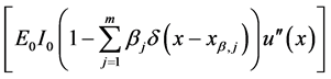
In the case of flexural stiffness, Equation (131), the governing Equation (129) takes the following form,

 (132)
(132)
where  and
and  are constants of integration and
  indicates a primitive of order k of the external load function
 .
.
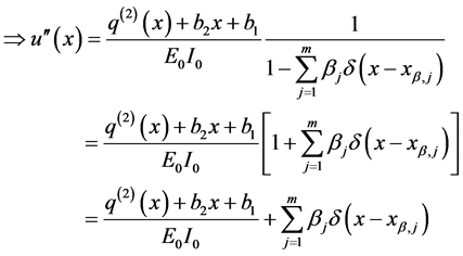
Using the properties of unit step function, Equation (132) can be rewritten as,

 (133)
(133)
where
 (134)
(134)
Equation (133) show that the flexural stiffness model given by Equation (131) provides a curvature function with jump discontinuities at ;
;  of the curvature function are dependent on the discontinuity intensities at
 ;
; .
.
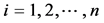
Integration of Equation (131) provides the slope function as follows:
 (135)
(135)
Integration of Equation (135) provides the following closed form expression for the deflection function
 (136)
(136)
Equation (135) and Equation (136) represents the generalization of multiple flexural stiffness discontinuities, of the type Equation (131), of the closed form expressions for a single discontinuity.
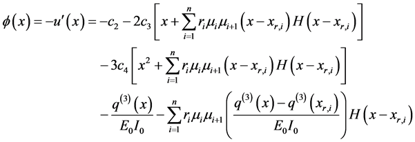
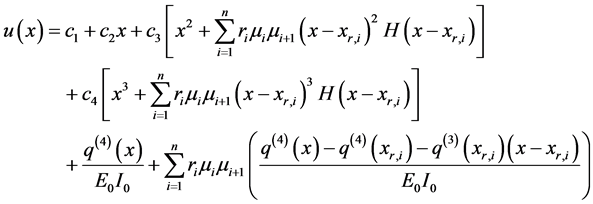
・ The bending moment function is obtained by multiplying the curvature function, Equation (133) by Equation (131), as follows:
 (137)
(137)
・ The shearing force function is obtained by differentiating Equation (137) as follows:
 (138)
(138)
Equation (137) and Equation (138) are for a single singularities and show that the flexural stiffness discontinuities do not appear explicitly. In fact, it is expected that bending moment  and shear force
  are independent of the flexural stiffness (for statically determinate beams). But, the discontinuity intensities
  and positions
  appear explicitly in the integration constants
 ,
,  (for statically determinate beams.)
7. Solutions of Euler-Bernoulli Beams in Presence of Multiple Slope Discontinuities
For the case of multiple slope discontinuities, we adopt a new technique of integration.
In the case of flexural stiffness provided by Equation (131), the governing Equation (129) takes the following form:
 (139)
(139)

 (140)
(140)
To solve the product of two Dirac’s delta distributions, we will rely on the technique proposed by Bagarello (1995; 2000) [9] . Bagarello indicates that the product of two Dirac’s deltas both centered at  can be reduced to a singe Dirac’s delta multiplied by a constant A as follows:
 (141)
(141)
where ; and
; and  is a test function.
Hence,
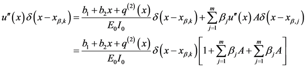
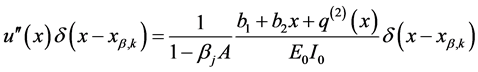 (142)
(142)
Substituting Equation (142) into Equation (140) given the following explicit expression of the curvature for the considered beam model
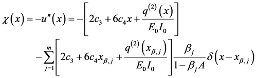 (143)
(143)
Integration of Equation (143) provides the following slope function showing discontinuities at the abscissa 
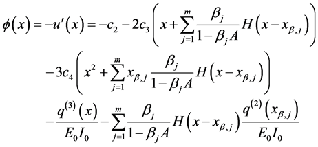 (144)
(144)
Further integration of Equation (144) provides the following closed form expression for the deflection function of the beam
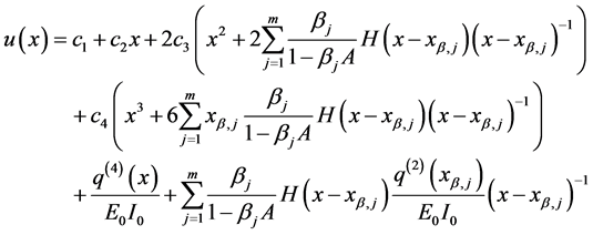 (145)
(145)
The bending moment and shear force function formally coincide with Equation (126) and Equation (128), respectively. In fact, for statically determine beams,  and
and  should not depend on the adopted flexural stiffness. On the contrary, for statically indeterminate beams, the adopted flexural stiffness model will affect the expressions of the constants
 ,
, .
.
The slope function defined in Equation (144) presents jump discontinuities  at
at  that are explicitly evaluated as follows:
 (146)
(146)
and comparison of Equation (146) with the bending moment given by Equation (126) evaluated at  leads to
 (147)
(147)
Equation (147) corresponds to the presence of internal hinges at ;
; , endowed with rotational springs with stiffness
  as shown in Figure 8(a), given as
 (148)
(148)
Since rotational spring stiffness can take values from zero (no rotational spring) up to infinity (continuous beam at , with no internal hinges), discontinuity values
 , in view of Equation (148), can take values from 0 up to 1.
However, if rotational spring stiffness , are assigned to the related value
  have to be obtained by Equation (148) for a value of the quantity A among those proposed by Bagereuo (1995) [9] .
Cite this paper
Chalishajar, D., States, A. and Lipscomb, B. (2016) On Applications of Generalized Functions in the Discontinuous Beam Bending Differential Equations. Applied Mathematics, 7, 1943- 1970. http://dx.doi.org/10.4236/am.2016.716160
References
- 1. Timoshenko, S. and Woinowsky-Kreiger, S. (1959) Theory of Plates and Shells. 2nd Edition, McGraw-Hill, New York.
- 2. Gorman, D.J. (2008) On the Use of the Dirac Delta Function in the Vibration Analysis of Elastic Structures. International Journal of Solids and Structures, 45, 4605-4614.
http://dx.doi.org/10.1016/j.ijsolstr.2008.03.009 - 3. Timoshenko, S.P. (1976) Strength of Materials: Part I. Krieger, Malabar.
- 4. Shames, I.H. (1989) Introduction to Solid Mechanics. Prentice-Hall, New York.
- 5. Kanwal, R.P. (1983) Generalized Functions Theory and Applications. Academic Press, New York.
- 6. Palmeri, A. and Cicirello, A. (2011) Physically-Based Dirac’s Delta Functions in the Static Analysis of Multi-Cracked Euler-Bernoulli and Timoshenko Beams. International Journal of Solids and Structures, 48, 2184-2195.
http://dx.doi.org/10.1016/j.ijsolstr.2011.03.024 - 7. Yavari, A., Sarkani, S. and Moyer, E.T. (2000) On Applications of Generalised Functions to Beam Bending Problems. International Journal of Solids and Structures, 38, 8389-8406.
http://dx.doi.org/10.1016/S0020-7683(01)00095-6 - 8. Yavari, A. and Sarkani, S. (2001) On Applications of Generalised Functions to the Analysis of Euler-Bernoulli Beam-Columns with Jump Discontinuities. International Journal of Mechanical Sciences, 43, 1543-1562.
http://dx.doi.org/10.1016/S0020-7403(00)00041-2 - 9. Bagarello, F. (1995) Multiplication of Distribution in One Dimension: Possible Approaches and Applications to Delta-Function and Its Derivatives. Journal of Mathematical Analysis and Applications, 196, 885-901.
http://dx.doi.org/10.1006/jmaa.1995.1449