Applied Mathematics
Vol.5 No.12(2014), Article
ID:47377,10
pages
DOI:10.4236/am.2014.512169
Numerical Approximation of Fractal Dimension of Gaussian Stochastic Processes
Freddy H. Marin Sanchez1, William Eduardo Alfonso2
Basic Science Department, EAFIT University, Carrera 49 # 7 Sur-50, Medellín, Colombia
Email: fmarinsa@eafit.edu.co, walfonso@eafit.edu.co
Copyright © 2014 by authors and Scientific Research Publishing Inc.
This work is licensed under the Creative Commons Attribution International License (CC BY).
http://creativecommons.org/licenses/by/4.0/


Received 27 March 2014; revised 30 April 2014; accepted 7 May 2014
ABSTRACT
In this paper we propose a numerical method to estimate the fractal dimension of stationary Gaussian stochastic processes using the random Euler numerical scheme and based on an analytical formulation of the fractal dimension for filtered stochastic signals. The discretization of continuous time processes through this random scheme allows us to find, numerically, the expected value, variance and correlation functions at any point of time. This alternative method for estimating the fractal dimension is easy to implement and requires no sophisticated routines. We use simulated data sets for stationary processes of the type Random Ornstein Uhlenbeck to graphically illustrate the results and compare them with those obtained whit the box counting theorem.
Keywords:Stationary Gaussian Stochastic Processes, Fractal Dimension, Random Euler Numerical Scheme

1. Introduction
A common practice when trying to measure irregular shapes, such as the perimeter of an island or the length of a coastline, is to use Euclidean geometry, ignoring the fact that these shapes do not correspond to the ones of ideal objects, such as polygons and circles, whose dimension is an integer. In contrast, many forms observed in nature have a special feature that makes their resulting measurement depend on the measuring scale, such that the lower the scale, the higher the value of the measurement, to the point where it becomes infinite or indeterminate. The dimension of irregular shapes is a non-integer dimension known as the Hausdorff-Besicovitch dimension. In the early twentieth century, Lewis Fry Richardson found a relationship that allows determining the value of a constant that indicates the degree of roughness of a coast or a geographical border, and used it to calculate the border length between several countries [1] . Based on Richardson’s findings, Benoit Mandelbrot [2] found that such irregular shapes have the property of statistical self-similarity, which states that any portion of an irregular shape can be considered a fully scaled image of the entire shape. Later, Mandelbrot coined this property as the fractal dimension to describe sets in . There are many studies in the literature in which maps, border areas and natural and physical phenomena are modeled and simulated with fractal features. In [3] for example, a proposal to simulate real maps using the fractal dimension of Gaussian stochastic processes is presented and some reports modeling terrestrial surfaces, irregular oceanic coasts and rivers, can be found in [4] -[9] .
There are several approaches to estimating of the fractal dimension. In fact in [10] different types of fractals that appear in scientific research are examined, application in nonlinear dynamical systems is discussed, and an exahustive review of numerical methods for their estimation is done.
[11] proposed another method for estimating the fractal dimension of subset of , as well as an additional correction to address the problem of resolution, allowing obtaining not only the fractal dimension, but also a confidence interval for this estimation, thus improving the box counting method. They also show some experimental results based on simulated data and real data from the coastline of Norway. The techniques for the measurement of fractal dimension can be divided into two groups: those based on vectors, which include structured algorithms, and those based on matrices, for the analysis of image systems that include the distance transformation method reported in [12] . Moreover, [13] introduces the roughness method in order to determine the fractal dimension of the Sierpinski carpet, triangle and tetrahedron, the standard Cantor set and the Menger sponge. Meanwhile, in the study of stochastic signals filtering by [14] is obtained the analytical formulation of the fractal dimension to investigate the effects of a linear filter and the regularity in a particular mono-fractal stochastic process, based on an explicit, continuous formulation, linking the spectral properties of a given filter and the fractal properties of a given process, knowing the function of probability density and output, departing from the correlation coefficient of the filter. With regard to the arguments established by [14] , the aim of our study is to estimate, numerically, the fractal dimension of ergodic stationary Gaussian stochastic processes using the random Euler scheme.
This paper is organized as follows. Section 2 presents the Euler random scheme and builds the numerical solution, the expected value and the crossed expected value for a more general stochastic processe that allows calculating the variance and correlation of the solution of problems of random initial value; the definition of fractal dimension and the box counting theorem are described in Section 3. In Section 4 we present a numericalanalytical formulation for calculating length and fractal dimension for stationary Gaussian stochastic processes. A method to calculate the length and fractal dimension of stationary Gaussian stochastic processes that include processes such as random Ornstein Uhlenbeck is presented in Section 5. Section 6 illustrates graphically, some experimental numerical results associated with the calculation of the fractal dimension of ergodic stationary Gaussian stochastic processes, compared with the results obtained from using the box count theorem.
2. On the Random Euler Numerical Scheme
Consider the initial random value problem of the form1,
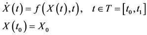 (1)
(1)
where  is a random variable and therefore
  as
as  are both unknown stochastic processes defined on the same probability space
 . The aim of this section is to use the Euler scheme to construct a numerical solution, the expected value and the crossed expected value to random initial value problem (1).
Note that the discretized solution of Equation (1) can be expressed in integral form as

By using the approximation , the numerical scheme
 (2)
(2)
is obtained, where ,
,  are second order random variables (2-r.v.) and
 .
.
In particular, consider a (2-r.v.)  and a stochastic process
  second order (2-s.p.) m.s. integrable defined on the same probability space
  such that
  is independent of
  for each
  lying in the interval
  Let
Let  a continuous deterministic function defined on
 . The idea is to solve numerically initial random value problems given by the expression
 (3)
(3)
Note that the Euler numerical scheme for problem (3)2 takes the form
 (4)
(4)
It is easy to show using the principle of mathematical induction, (see [19] and [20] pp. 58-59), that  and
and  can be expressed as
 (5)
(5)
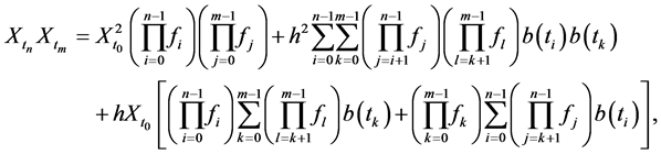 (6)
(6)
where . From Equations (5), (6) and the results reported in [19] , it follows that the expected values
  and
and  takes the form
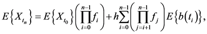 (7)
(7)
 (8)
(8)
3. Fractal Dimension and the Box Counting Theorem
The fractal dimension is an objective way to compare fractals geometrically. This section introduces the concept of fractal dimension and presents the box counting theorem.
Let  denote a complete metric space. Let
  be a nonempty compact subset of
![]() . Let
. Let  denote the closed ball of radius
 ![]() and center at a point
and center at a point![]() . We wish to define an integer,
. We wish to define an integer,  , to be the least number of closed balls of radius
  needed to cover the set
 ![]()
That is, : smallest positive integer
  such that
 , for some set of distinct points
  In other words, surround every point
 ![]() by an open ball of radius
by an open ball of radius ![]() to provide a cover of
to provide a cover of  by open sets. Because
  is compact this cover possesses a finite subcover, consisting of an integer number, say
 , of open balls. By taking the closure of each ball, thus obtained a cover consisting of
  closed balls. Let
 ![]() denote the set of covers of
denote the set of covers of  by at most
  closed balls of radius
 . Then
 ![]() contains at least one element.
contains at least one element.
Let  defined by
  number of balls in the cover
![]() . Then
. Then  is a finite set of positive integers. It follows that it contains a least integer,
 .
.
The intuitive idea behind fractal dimension is that a set  has fractal dimension
 ![]() if:
if: ![]() for some positive constant
for some positive constant ![]() 3.
3.
Accordingly,

Now notice that the term  approaches 0 as
![]() . This leads us to the following definition.
. This leads us to the following definition.
Definition 3.1. Let  where
where  is a metric space. For each
![]() , let
, let  denote the smallest number of closed balls of radius
 ![]() needed to cover
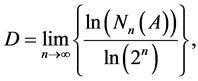
needed to cover . If
. If

exists, then ![]() is called the fractal dimension
is called the fractal dimension . Also used the notation
  and will say “
 has fractal dimension
![]() ”.
”.
Theorem 3.2. The Box Counting Theorem. Let , where the Euclidean metric is used. Cover
  by closed square boxes of side length
 . Let
. Let  denote the number of boxes of side length
  which intersect the attractor. If
then  has fractal dimension
![]() . The proof of this theorem and other important definitions can be found at [21] .
. The proof of this theorem and other important definitions can be found at [21] .
4. Analytical Formulation of the Fractal Dimension for Stochastic Processes
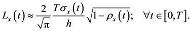
An analytical expression for the fractal dimension of filtered stochastic signals with the purpose of studying the effects of a linear filter and the regularity of a given stochastic mono-fractal process is introduced in [14] . They present some arguments using the Euclidean length of a deterministic curve  with limited duration
 , as starting point to estimate the length and fractal dimension of such stochastic signals.
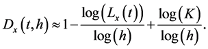
However, stochastic processes can not be described by deterministic continuous curves and irregularities are present even when examined with higher resolutions. This leads to the paradoxical conclusion that the lengths of such signals are not finite. To overcome the fact that stochastic processes lack of a finite longitude, [2] assumes that the longitude  of a fractal curve depends on the resolution and the length of the measurement instrument,
![]() . [1] proves that measuring
. [1] proves that measuring  as a function of
 ![]() allows to determine the fractal dimension i.e.:
allows to determine the fractal dimension i.e.:
![]() (9)
(9)
where  is the fractal dimension of the curve and
  is a constant.
Thus, the length  can be written as a function of
 ![]() given by
given by
 (10)
(10)
where  and where the elementary length is given by
 .
.
This definition of length for continuous curves can be extended to ergodic stationary stochastic processes by replacing the arithmetic mean by the mathematical expectation , i.e.

where .
.
Note that  only is solved numerically. In particular, for a high frequency sampling it can be assumed that
  to obtain an analytical expression given by [22]
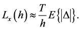 (11)
(11)
Length and Fractal Dimension for Gaussian Stochastic Processes
Following the results reported in [14] , we will make a brief extension that also requires a prior information such as the probability density function of the process and the variance and correlation functions.
Consider a stochastic process ![]() with values in
with values in  defined on a probability space
 . The average length of the process can be estimated by the expression
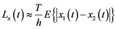 (12)
(12)
with . Thus, the expected value of the absolute value of the difference between
  and
and  takes the form
 (13)
(13)
where,  denotes the joint probability density function.
Now suppose that the stochastic process ![]() is a stationary Gaussian process. Consequently,
is a stationary Gaussian process. Consequently,  and
and  are also Gaussian stationary and therefore the joint probability density can be written as
 (14)
(14)
where ![]() and
and ![]() are the variances of
are the variances of  and
and  respectively, and
  is the correlation function defined by
 .
.
The probability density of the increment  is
is
 (15)
(15)
Analogously to [14] , the probability density of the increment follows a normal distribution :
:
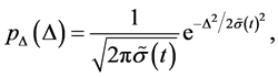 (16)
(16)
with . As
. As  and
and  belong to the same process
![]() then
then  and the standard deviation is
The mathematical expectation of the increment becomes
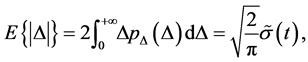 (17)
(17)
and thus
 (18)
(18)
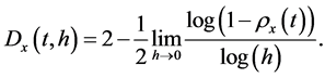
Using Equation (9), the fractal dimension  of the process
 ![]() can be approximated as
can be approximated as
 (19)
(19)
Finally, Equation (18) becomes
 (20)
(20)
5. Numerical Approach to Fractal Dimension for Stationary Gaussian Processes
In this section we present the numerical construction of the fractal dimension for stationary Gaussian stochastic processes including random Ornstein Uhlenbeck process, using the results of Section 4, the random Euler numerical scheme and the approximation of correlation function using the calculations for  and
and  described in Section 2.
5.1. Calculation of Fractal Dimension for the Random Ornstein Uhlenbeck Process
Consider the random initial value problem given by
![]() (21)
(21)

where![]() ,
, ![]() , and
, and  is a Gaussian white noise independent of
  for each
  lying in the interval
  (defined as in [16] p. 121) and
 . Note that this process is stationary Gaussian and ergodic, and can be considered as a modification of the random walk in continuous time and analog to the order 1 autoregressive process, AR (1) with discrete time, that broadly describes the velocity of a Brownian mass particle under the influence of friction [23] .
Under random Euler numerical scheme (5), the Equation (21) can be expressed as
 (22)
(22)

where . By Equation (8) it follows that

Trivially note that . For
. For ,
, ; thus

For the case in which ![]() and
and ![]() it follows that
it follows that

It is easy to see that , and
, and . In this way,

which by Equation (20) becomes
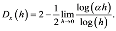 (23)
(23)
5.2. Calculation of Fractal Dimension for a Random Mean Reverting Process
Consider the random initial value problem given by
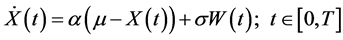 (24)
(24)

where![]() ,
, ![]() ,
,  ,
,  is a Gaussian white noise independent of
  for each
  lying in the interval
  (defined as in [16] p. 121) and
  with
with . Note that this process is stationary Gaussian and ergodic. When the initial condition is constant, this process is also known as mean reversion process with additive noise. This kind of process has been widely used in modeling the dynamic behavior of commodity prices and short term interest rates (see [24] and references therein), and the simulating of realistic irregular lattices in [3] .
Equation (24) can be written as
![]() (25)
(25)
Under random Euler numerical scheme, Equation (25) can be expressed as
 (26)
(26)

Equation (8) implies that for  and
and ,
,

Note that for ,
, ; in this way,
 .
.

For the case in which ![]() and
and ![]() it follows that
it follows that .
.
It is easy to see that  and
and
 . In this way,
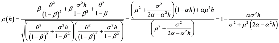
Equation (20) becomes
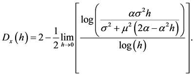 (27)
(27)
6. Numerical Results
This section graphically illustrates some experimental numerical results related to the calculation of the fractal dimension for stationary Gaussian stochastic processes associated with random initial value problems (21) and (24).
Figure 1(a) shows a comparison between the approximate average fractal dimension of 1000 simulated trajectories for Ornstein Uhlenbeck process using the Box Counting theorem and the numerical fractal dimension proposed in Equation (23) for different values of . In Figure 1(b) the dynamic behavior of the fractal dimension is shown for different values of the parameter
 .
.
Figure 2(a) shows a comparison between the approximate average fractal dimension of 1000 simulated
 (a)
(a) (b)
(b)
Figure 1. (a) Numerical comparison of fractal dimension for Ornstein Uhlenbeck processes with ,
, ![]() and
and ![]() for different values of
for different values of![]() ; (b) Dynamic behavior of the fractal dimension for Ornstein Uhlenbeck processes with
; (b) Dynamic behavior of the fractal dimension for Ornstein Uhlenbeck processes with ,
,  and
and ![]() for
for![]() .
.
 (a)
(a)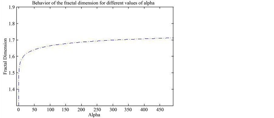 (a)
(a)
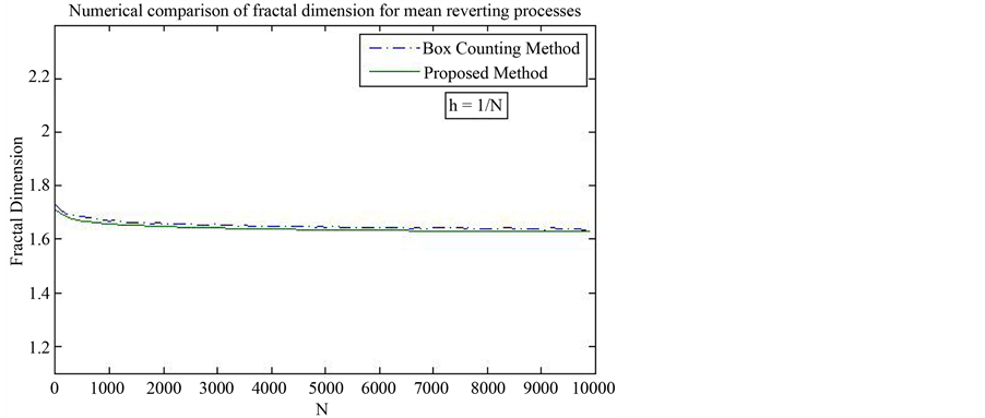
Figure 2. (a) Numerical comparison of fractal dimension for mean reverting processes with ,
,  ,
, ![]() and
and ![]() for different values of h; (b) Dynamic behavior of the fractal dimension for mean reverting processes with
for different values of h; (b) Dynamic behavior of the fractal dimension for mean reverting processes with ,
,  ,
,  and
and ![]() for
for![]() .
.
trajectories for mean reverting process using the Box Counting theorem and the numerical fractal dimension proposed in Equation (27) for different values of . In Figure 2(b) the dynamic behavior of the fractal dimension is shown for different values of the parameter
 .
.
7. Conclusions
This paper made a slight extension of the approach proposed in [14] for the numerical estimation of the fractal dimension of ergodic stationary Gaussian stochastic processes associated with the random Ornstein Uhlenbeck process. Using random Euler scheme performed numerical construction of the expectation value, variance and correlation functions at any point of time to initial random value problems general. The computational implementation of this alternative method to estimate the fractal dimension is easy and requires no sophisticated routines. It illustrates graphically the results obtained compared with box counting theorem using simulated data sets for stationary processes type random Ornstein Uhlenbeck.
A clear convergence of the proposed methods is shown in Figure 1(a) and Figure 2(a). In addition, the results show that the fractal dimension of Ornstein Uhlenbeck processes is independent of the parameter![]() . This independence is maintained in the mean reverting process for the case where
. This independence is maintained in the mean reverting process for the case where . Figure 1(b) and Figure 2(b) reflect the fact that the fractal dimension of this type of process is more sensitive to the parameter
 .
.
References
- Richardson, L. (1961) The Problem of Contiguity: An Appendix of Statistic of Deadly Quarrels. General Systems Year Book, 61, 139-187.
- Mandelbrot, B. (1967) How Long Is the Coast of Britain Statistical Self-Similarity and Fractional Dimension. Science, 156, 636-638. http://dx.doi.org/10.1126/science.156.3775.636
- Duque, J.C., Betancourt, A. and Marin, F. (2014) An Algorithmic Approach for Simulating Realistic Irregular Lattices. In: Thill, J.C. and Dragicevic, S., Eds., GeoComputational Analysis and Modeling of Regional Systems, Springer Heidelberg, in press.
- Mandelbrot, B. (1975) Stochastic Models for the Earth’s Relief, the Shape and the Fractal Dimension of the Coastlines, and the Number-Area Rule for Islands. Proceedings of the National Academy of Sciences, 72, 3825-3828. http://dx.doi.org/10.1073/pnas.72.10.3825
- Adler, R.J. (1978) Some Erratic Patterns Generated by the Planar Wiener Process. Advances in Applied Probability, 10, 22-27. http://dx.doi.org/10.2307/1427003
- Cullin, W.E. and Datko, M. (1987) The Fractal Geometry of the Soil-Covered Landscape. Earth Surface Processes and Landforms, 12, 369-385. http://dx.doi.org/10.1002/esp.3290120404
- Cullin, W.E. (1988) Dimension and Entropy in the Soil-Covered Landscape. Earth Surface Processes and Landforms, 13, 619-648. http://dx.doi.org/10.1002/esp.3290130706
- Beauvais, A. Montgomery, D. (1996) Influence of Valley Type on the Scaling Properties of River Planforms. Water Resources Research, 32, 1441-1448. http://dx.doi.org/10.1029/96WR00279
- Montgomery, K. (1996) Sinuosity and Fractal Dimension of Meandering Rivers. Area, 28, 491-500.
- Theiler, J. (1990) Estimating Fractal Dimension. JOSA A, 7, 1055-1073. http://dx.doi.org/10.1364/JOSAA.7.001055
- Taylor C. and Taylor, S.J. (1991) Estimating the Dimension of a Fractal. Journal of the Royal Statistical Society. Series B (Methodological), 53, 353-364.
- Allen, M., Brown, G.J. and Miles, N.J. (1995) Measurement of Boundary Fractal Dimensions: Review of Current Techniques. Powder Technology, 84, 1-14. http://dx.doi.org/10.1016/0032-5910(94)02967-S
- Blachowski, A. and Ruebenbauer, K. (2009) Roughness Method to Estimate Fractal Dimension. Acta Physica Polonica A, 115, 636-640.
- Girault, J., Kouame, D. and Ouahabi, A. (2010) Analytical Formulation of the Fractal Dimension of Filtered Stochastic Signals. Signal Processing, 90, 2690-2697. http://dx.doi.org/10.1016/j.sigpro.2010.03.019
- Loeve, M. (1963) Probability Theory. D. Van N. Company, London.
- Soong, T. (1973) Random Differential Equations in Science and Engineering. Academic Press, New York.
- Jodar, L., Cortez, J. and Villafuerte, L. (2007) Mean Square Numerical Solution of Random Differential Equations: Facts and Possibilities. Computers and Mathematics with Applications, 53, 1098-1106. http://dx.doi.org/10.1016/j.camwa.2006.05.030
- Jodar, L. and Villafuerte, L. (2007) Numerical Solution of Random Differential Equations: A Mean Square Approach. Mathematical and Computer Modelling, 45, 757-765. http://dx.doi.org/10.1016/j.mcm.2006.07.017
- Marin, F. and Laniado, H. (2014) Convergence of Analytical Stochastic Processes in Mean Square. 1-9. http://repository.eafit.edu.co/handle/10784/1523
- Agarwall, R. (1992) Difference Equations and Inequalities. Marcel Dekker, New York.
- Barnsley, M. (1988) Fractals Everywhere. Academic Press, London.
- Le Tavernier, E. (1998) La methode de Higuchi pour la dimension fractal. Signal Processing, 65, 115-128. http://dx.doi.org/10.1016/S0165-1684(97)00211-9
- Uhlenbeck, G. and Ornstein, L. (1930) On the Theory of the Brownian Motion. Physical Review, 36, 823-841. http://dx.doi.org/10.1103/PhysRev.36.823
- Marin, F. and Palacio, J. (2013) Gaussian Estimation of One-Factor Mean Reversion Processes. Journal of Probability and Statistics, 2013, 10 p.
NOTES

1See for details of second-order random variables (2-r.v.), second-order stochastic processes (2-s.p.), and random differential equations.

2Some convergence criteria random Euler scheme in the mean square sense can be viewed at -.

3The notation  as follows.
 , where
  and
and  be real valued functions of the positive real variable
 .
.