Applied Mathematics
Vol.5 No.5(2014), Article ID:44071,10 pages DOI:10.4236/am.2014.55079
Comparison of Machine Learning Regression Methods to Simulate NO3 Flux in Soil Solution under Potato Crops
J. G. Fortin1*, A. Morais1, F. Anctil1, L. E. Parent2
1Department of Civil and Water Engineering, Université Laval, Québec, Canada
2Department of Soils and Agrifood Engineering, Université Laval, Québec, Canada
Email: *jerome.goulet-fortin.1@ulaval.ca
Copyright © 2014 by authors and Scientific Research Publishing Inc.
This work is licensed under the Creative Commons Attribution International License (CC BY).
http://creativecommons.org/licenses/by/4.0/


Received 21 December 2013; revised 21 January 2014; accepted 28 January 2014
ABSTRACT
Nitrate (NO3) leaching is a major issue in sandy soils intensively cropped to potato. Modelling could test the effect of management practices on nitrate leaching, particularly with regard to optimal N application rates. The NO3 concentration in the soil solution is well known for its local heterogeneity and hence represents a major challenge for modeling. The objective of this 2-yearstudy was to evaluate machine learning regression methods to simulate seasonal NO3 concentration dynamics in suction lysimeters in potato plots receiving different N application rates. Four machine learning function approximation methods were compared: multiple linear regressions, multivariate adaptive regression splines, multiple-layer perceptrons, and least squares support vector machines. Input candidates were chosen for known relationships with NO3 concentration. The best regression model was obtained with a 6-inputs least squares support vector machine combining cumulative rainfall, cumulative temperature, day of the year, N fertilisation rate, soil texture, and depth.
Keywords:Machine Learning Regression; Nitrate Leaching; Suction Lysimeter; Potato Cropping System

1. Introduction
Groundwater nitrate (NO3) contamination is particularly common in sandy soils intensively cropped to potato or other high-N demanding crops. Estimates of the apparent recovery of N fertiliser in the potato plant in Quebec ranged between 29% - 70% in loamy sands [1] and 21% - 62% in sandy soils [2] . Modeling could test the effect of management practices on nitrate leaching, particularly with regard to optimal N application rates.
Process-based NO3 models require local soil, climatic, and management data as input, which are generally not available unless model calibration is the main intent [3] . Alternative approaches using empirical relationships between N soil status and surrogate variables may therefore fill that gap. Machine learning is one of the most important and useful data mining tools that can reveal non-linear interactions and patterns among data sets.
The objective of this study was to compare machine learning regression methods to simulate the seasonal dynamics of daily NO3 flux (NF) from surrogate input variables. Four methods were evaluated: multiple linear regression (MLR) used here as reference model, multivariate adaptive regression splines (MARS), multiple-layer perceptrons (MLP), and least squares support vector machines (LS-SVM). Input candidates were selected for their known relationships with NF: N fertilization rate (Nfert), cumulative rainfall (Σrain), cumulative temperature (Σtemp), day of the year (DOY), percentage of clay (% Clay), and soil depth (depth). The NO3 losses in kg NO3·ha−1are generally computed as the integral of the curve relating concentration to cumulative water loss [4] . Only NO3 concentration was considered in this study.
2. Material and Method
The meteorological data were obtained at a daily time-step from a nearby micro-meteorological station from planting to harvest. In most N and C models, the minimum climatic input data requirement for simulating soil biological activity includes precipitation, temperature, and information on potential (or open pan) evapotranspiration. Because soil organic matter mineralization into inorganic N forms shows reportedly little sensitivity to evapo transpiration [5] , only cumulative temperature and cumulative precipitation were considered.
Soil NO3 concentration data were collected from 4rainfedpotato (Solanum tuberosum L.) fields located at Groupe Gosselin FG Inc. near Pont Rouge, Québec, Canada (Lat. 46˚45'N; Long. 71˚42'W). Each site was divided into three large blocks submitted to the following N treatments at planting: 0, 90, 130, and 170 kg·N·ha−1. Soils were sampled in the spring at each site to determine particle-size distribution using the hydrometer method [6] . Suction lysimeters (model 1900L24-B02M2, Soil Moisture Equipment Corp., Ca) were installed into soil at planting. There were 3 replications per treatment, for a total of 36 lysimeters. Extraction of soil water from suction lysimeters was performed about 7 - 8 times each year. The NO3 concentration of the solution was determined by liquid chromatography using a Dionex ICS2000 equipped with a UV-detector (Dionnex Corporation, Synnyvale, Ca). For each treatment, the results of 3 replications were averaged prior to modeling.
2.1. The Regression Models
2.1.1. Multiple Linear Regression
Multiple linear regression (MLR) was used as a reference model because of its simplicity and wide usage. It relates p explanatory variables x to NF at each time step t by fitting a linear equation to the data [7] :
 (1)
(1)
where dNF/dt is a  column vector (n = number of sampling occasions), X is a
  matrix, b is a
  column vector (the intercept bo and the slopes bp), and
  is a
is a  vector of residuals that followsa multivariate normal distribution with mean of 0 and covariance matrix of
 , where I is the identity matrix. The regression coefficient
  reflects the partial effect of x1(x2) when x2(x1) is held constant:
 (2)
(2)
2.1.2. Multivariate Adaptive Regression Splines
The multivariate adaptive regression splines (MARS) simulates NF seasonal dynamics with M basis functions as follows [8] :
 (3)
(3)
where c0 is a constant,  is the mth basis function and cm is coefficient of the mth basis functions. MARS builds a model in two stages as forward and backward passes [9] [10] . During the forward pass, the algorithm starts with a “no-knowledge” model (i.e. the average response values at each time-step). Afterwards, the algorithm adds basis functions in pairs to the model. At each step, it finds the pair of functions producing maximum reduction of the error term. The two functions in the pair are identical except that a different side of a mirrored hinge function is used for each function. The addition of basis functions continues until the change in residual error becomes sufficiently small or until a pre selected maximum number of basis functions set sis reached. To avoid over-fitting, the backward pass prunes the model. It removes basis functions one by one, deleting the least effective ones at each step until it finds the best sub-model.
In order to determine which basis functions should be included in the model and to secure model generalization capacity, MARS exploits a generalized cross validation (GCV) [11] [10] : the mean squared residual error divided by a penalty depending on model complexity. The GCV criterion is defined as follows [12] :
 (4)
(4)
where C(M) is a complexity penalty that increases with the number of basis functions in the model [9] :
 (5)
(5)
where M is the number of basis functions in Equation (3) and d is a penalty for each basis function included in the model. It can be also regarded as a smoothing parameter. During this study, all MARS models were built using the ARES lab toolbox ver.1.5.1 [13] .
2.1.3. Multiple-Layer Perceptron
Multiple-layer perceptron networks (MLPs) are also considered. They consist in a single layer of hidden neurons and a single output neuron. The MLP function of NF must be optimized at each time step across the following linear combination of multivariate functions:
 (6)
(6)
where x is an ith-dimensional input vector, j is number of hidden neurons,  are neural weights, and
  are neural biases. The sigmoid tangent activation function G1 and the linear activation function G2 were computed as follows [14] :
 (7)
(7)
 (8)
(8)
where  is the weighted sum of information from the previous layer of neurons.
Stacking [15] was selected to support MLP’s generalization. This method calibrates several networks of the same architecture and simulates NF by calculating the mean of the responses across networks.
2.1.4. Least Squares Support Vector Machine
In SVM regression, the inputs are mapped in an m-dimensional feature space using some fixed (nonlinear) mapping, and a linear model is built in this feature space. Mathematically, it is given by [11] :
 (9)
(9)
where X is the input vector,  the SVM weights vector,
  denotes a set of nonlinear transformations, and
  is the bias. The algorithm performs regression in the high-dimension feature space using the
  -insensitive loss as cost function (see [11] , for details) and, simultaneously, reduces model complexity minimizing
 . This can be described by introducing the non-negative slack variables
  and
and  that measure the deviation of the n training samples outside the
  -insensitive zone (also named
  -tube). The SVM regression is thus formulated as a minimization of the following functional:
 (10)
(10)
 (11)
(11)
where the constant C > 0 determines the trade-off between the complexity of the model (flatness) and up to what deviations larger than  are tolerated. Equation (11) implies that only data outside the
  -tube (i.e. “support vectors”) will be used in model building. This optimization problem can be transformed into a dual problem (see [16] , for details) and its solution is given by:
 (12)
(12)
where nsv is the number of support vectors,  are Lagrange multipliers, and K is a specified kernel function that measures the non-linear dependence between two instances of the input variables. Examples of kernel functions commonly used by SVMs are polynomial, radial basis, and sigmoid.
Least squares support vector machine (LS-SVM) is a reformulation of SVM. The LS-SVM uses a least squares loss function instead of the  -insensitive loss function. It is known to be easier to optimize with shorter computational time [17] . In LS-SVM, the
  -tube and slack variables are replaced by error variables, which inform on the distances from each point to the regression function. All samples in LS-SVM are therefore support vectors, i.e. all training data are used to build the model. The regularization constant C (which was related to the
  -tube) is replaced by γ, determining the trade-off between the fitting error minimization and smoothness of the estimated function. Although the choice of kernel functions is the same as SVM, LS-SVM generally uses the radial basis function, which is defined as follow:
 (13)
(13)
where  is a width parameter. The γ and
  parameters have to be determined by the user. All LS-SVM regression models were performed using the LS-SVM lab toolbox [18] .
2.2. Model Calibration
The available 14 field plots were split into training and validation datasets; 65% of them were selected to train the model while the remaining was used for validation. To ensure statistical homogeneity between the training and testing datasets, a (1-d) Kohonen self-organizing feature map (KSFOM) [19] was constructed with maximal seasonal NF’s as input.
Input variables selection is a typical problem for machine learning. As the a priori knowledge of the problem led us considering few entries, a sequential forward selection was chosen for its simplicity. In sequential forward selection, the model inputs are first tested individually. Thereafter, following a stepwise method, combinations with an increasing number of variables are tested. The process stops when the addition of further variable stops increasing model’s performance. A first sequential forward selection was operated with a given set of model parameters. Once the best combination of variable was found, these parameters were optimized and a second sequential forward selection was done to ascertain that the best combination of variable did not change with the new parameter values. Only the performance obtained with the optimized parameters are presented here.
2.3. Evaluation
Model performance was evaluated calculating the Mean Absolute Error (MAE) and the Root Mean Square Error (RMSE) on NF—see [20] for details about these linear scoring rules.
The scale dependency of the linear scoring rules can be overcome using a skill score: a simple score standardization method that compares the performance of the simulation with that of a reference simulation. The NashSutcliffe efficiency index (NS) was use to this purpose [21] . A NS of 1 represents a perfect fit between simulated and observed values, while a NS of 0 is equivalent to a “no-knowledge” model, namely the mean of observations at every time step. Since scoring rules are averaged across the dataset, scatter plots are also drawn and regression lines are computed to visually assess the concordance and bias between simulated and observed NF.
3. Results and Discussion
Figure 1 presents the measured seasonal NF for all plots for the 2 seasons of the study. Because some of the lysimeters did not retain their tension in 2012, the 0 and 90 kg·N·ha−1 treatments were only represented for one of the 2 sites in the first year. Note that all lysimeters did not collect water at every sampling time, explaining the disparities between time-series. The seasonal dynamics is generally characterized by a NF peak following N application at planting. As plants grew and took up nitrates, NF generally decreased as reported in previous studies (e.g. [22] ). Averaged NF of the 32 operational lysimeters over the entire season of measure was145 mg NO3·L−1, which is comparable to reported NF for sandy soil under potato in Quebec [23] [24] . A loose relationship between N treatment and NF can be observed at Figure 1 (coefficient of correlation = 0.33). Higher maximal seasonal NFs were obtained with treatments of 130 and 170 kg·N·ha−1 and the 0 treatment generally show low NF values. However, this relationship was not linear. For instance, one of the 170 kg·N·ha−1treatment in 2013 presented very low maximal NF while a 0 treatment presented relatively high NF in 2012 possibly due to stimulated and impaired growth patterns, respectively. This suggests that other explicative variables are required to reliably assess NF.
3.1. Modelling of NO3 Flux Concentration
Statistics on models’ performance in training are presented in Table 1, while Table 2 presents statistics on selected model performance for validation. The best MLR model was retained as reference (for brevity, only the best MLR is presented in Table 2). It contains input variable candidates, namely Σrain, DOY, Σtemp, Nfert, depth and %clay. The NS reached 0.33 in training, with MAE of 79.2 mg NO3 L−1 (50.0% of the mean NFvalue of the calibration samples). Performance on testing, however, revealed complete absence of generalisation capacity of the linear approach. Figure 2(a) presents the scatter plot of observed and simulated NF using the best MLR during training and validation. Bias was close to 3000 mg NO3 L−1 during validation.
3.1.1. Multivariate Adaptive Regression Splines
For MARS, the variable explaining most variance was Σrain (NS = 0.24 in training), suggesting the importance of seasonal rainfall on NO3 leaching. The DOY and Σtemp also appeared influential with NS of about 0.2 in training. Depth and % clay did not weighted much at this step of the calibration. A 2-inputs MARS combining DOY and Σrain increased NS to 0.34in training. The addition of Σtemp and Nfert further increased performance, as suggested by the relationship between NFC and Nfert in Figure 1. The NS was 0.54 in training and the model
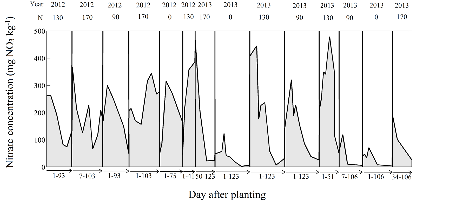
Figure 1.Seasonal dynamic of the measured NO3 concentration (mg NO3·L−1).

Table 1. Statistics of model performance during training.
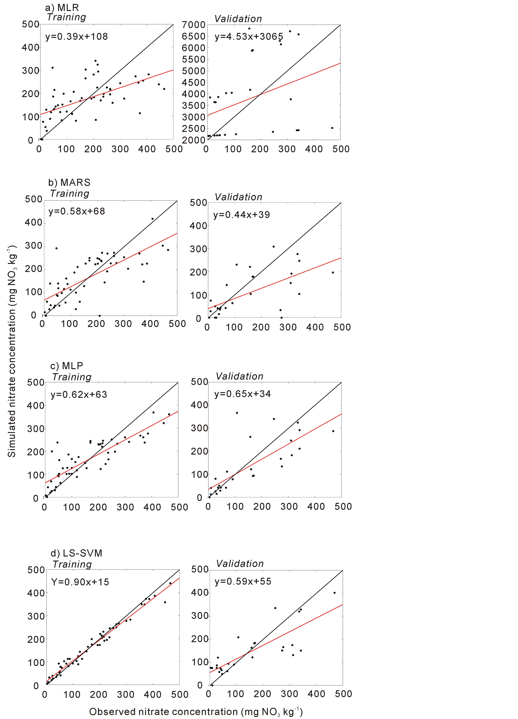
Figure 2. Scatter plot of the measured and simulated NO3 concentration (mg·NO3·L−1). The black line indicates the 1:1 line (perfect fit).
Table 2. Statistics of the selected model performance during validation.
was able to explain about 30% more variance than the reference model (r2 = 0.3). Further addition of depth and % clay did not improve model’s performance. Even though the generalisation capacity was highly improved as compared to MLR, it remained low with NS of 0.28 in validation. Figure 2(b) presents the scatter plot of observed and simulated NF using the best 4-inputs MARS. Compared to the reference model, the regression lines were closer to 1:1 and the intercept closer to 0, but scattering remained high especially in validation. The optimal maximal number of basis functions was 11.
3.1.2. Multiple-Layer Perceptron
Performances of the 1 to 3 inputs MLPs were similar to those of the MARS models. The main difference between these approaches was that the addition of depth and % clay substantially increased MLP performance. A 5-inputs MLP combining Σrain, DOY, Σrain, Nfert and % clay yielded NS of 0.77 in training. The generalisation capacity of the model appeared relatively good compared to the reference model, with NS of 0.52. The gain in performance over the linear model was substantial (r2 = 0.65). The scatter plot of the best 5-inputs MLP (Figure 2(c)) showed better fit than the best MARS, particularly in validation. The optimal number of hidden nodes was 3.
3.1.3. Least Squares Support Vector Machine
The optimal values for LS-SVM parameters γ and  were 11 and 1.1, respectively, compared to default values of 10 and 0.3 suggested in the LS-SVM lab toolbox. This larger
  indicates that more relative weights were given to points with larger distance from the regression function.
The 1 to 3 inputs LS-SVMs performed similarly as MARS and MLP. However, compared to MLP, the LS-SVMs showed higher sensitivity to depth and % clay. In training, NS of the best 6-input models (combining all input candidates) reached 0.95, with MAE as low as 15.9 mg NO3 kg−1 (10% of the mean NF value of the training dataset). Mean bias appeared significantly smaller than what was obtained in a previous study on potato fields within the same geographical location using transfer functions [24] . As expected, performance considerably decreased in validation, but less than the previous methods. The NS was 0.65 and MAE was 58.2 mg NO3 kg−1 (46% of the mean NF value of the validation dataset). Figure 2(d) revealed the very close fit of the 6-inputs LS-SVM in training. In calibration, however, the bias was higher than MLP, even though the scattering was slightly narrower.
These results suggests that the proposed 6-inputs LS-SVM performed best for general diagnostic of N leaching risk considering soil texture, local meteorological condition and N fertilisation rates. Further inclusion of spatial surrogate variables at field level (ex: leaf area index) could contribute reducing the error even more. Figure 3 presents the architecture of the final LS-SVM model and its general expression.
4. Conclusion
This study highlighted the non-linearity of NO3 flux in the soil solution and the need to rely on non-linear regression methods for its characterization. The best regression model was obtained with a 6-input least squares support vector machine combining cumulative rainfall, cumulative temperature, day of the year, N fertilisation
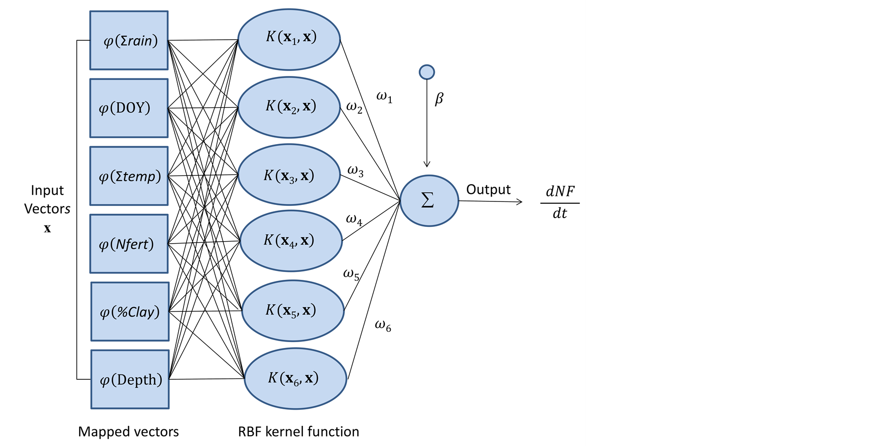
Figure 3.Architecture of the final 6-input LS-SVM and its general expression.
rate, soil texture, and depth. Performance in validation is satisfying considering the challenge that represents the NO3 flux concentration modeling of the soil solution. Further addition of spatial surrogate variables such as the leaf area index could improve the generalisation capacity of the model.
Acknowledgements
This project was funded by the Natural Sciences and Engineering Council of Canada (CRDPJ 385199-09) and the following cooperative partners: Cultures Dolbec Inc. (St-Ubalde, Québec), Groupe Gosselin FG Inc. (Pont Rouge, Québec), Agriparmentier Inc. (Notre-Dame-du-Bon-Conseil, Québec), and Ferme Daniel Bolduc et Fils Inc. (Péribonka, Québec).
References
- Li, H., Parent, L.-E., Karam, A. and Tremblay, C. (2003) Efficiency of Soil and Fertilizer Nitrogen of a Sod-Potato System in the Humid, Acid and Cool Environment. Plant and Soil, 251, 23-26. http://dx.doi.org/10.1023/A:1022983830986
- Cambouris, A.N., Zebarth, B.J., Nolin, M.C. and Laverdière, M.R. (2008) Apparent Fertilizer Nitrogen Recovery and Residual Soil Nitrate under Continuous Potato Cropping: Effect of N Fertilization Rate and Timing. Canadian Journal of Soil Science, 88, 813-825. http://dx.doi.org/10.4141/CJSS07107
- Jiang, Y., Zebarth, B.J., Somers, G.H., MacLeod, J.A. and Savard, M.M. (2012) Nitrate Leaching from Potato Production in Eastern Canada. In: He, Z., Larkin, R.P. and Honeycutt, C.W., Eds., Sustainable Potato Production: Global Case Studies, Springer, The Netherlands, 233-250. http://dx.doi.org/10.1007/978-94-007-4104-1_13
- Lord, E.I. and Shepherd, M.A. (1993) Development in the Use of Porous Ceramic Cum for Measuring Nitrate Leaching. Journal of Soil Science, 44, 435-449. http://dx.doi.org/10.1111/j.1365-2389.1993.tb00466.x
- Fortin, J.G., Bolinder, M.A., Anctil, F., Kätterer, T., Andrén, O. and Parent, L.-E. (2011) Effects of Climatic Data Low-Pass Filtering on the ICBM Temperatureand Moisture-Based Soil Biological Activity Factors in a Cool and Humid Climate. Ecological Modelling, 222, 3050-3060. http://dx.doi.org/10.1016/j.ecolmodel.2011.06.011
- Sheldrick, B.H. and Wang, C. (1993) Particle Size Analysis. In: Carter, M.R., Ed., Soil Sampling and Methods of Analysis, Lewis Publishers, Boca Raton, 499-517.
- Rosner, B. (2006) Fundamentals of Biostatistics. Duxbury Press, Boston, 6th Edition.
- Friedman, J.H. and Roosen, C.B. (1995) An Introduction to Multivariate Adaptive Regression Splines. Statistical Methods in Medical Research, 4, 197-217. http://dx.doi.org/10.1177/096228029500400303
- Friedman, J.H. (1991) Multivariate Adaptive Regression Splines. Annals of Statistics, 19, 1-141. http://dx.doi.org/10.1214/aos/1176347963
- García Nieto, P.J., Martínez Torres, J., de Cos Juez, F.J. and Sánchez Lasheras, F. (2012) Using Multivariate Adaptive Regression Splines and Multilayer Perceptron Networks to Evaluate Paper Manufactured Using Eucalyptus globulus. Applied Mathematics and Computation, 219, 755-763. http://dx.doi.org/10.1016/j.amc.2012.07.001
- Vapnik, V. (1998) Statistical Learning Theory. Wiley-Interscience, New York.
- Chou, S.M., Lee, T.S., Shao, Y.E. and Chen, I.F. (2004) Mining the Breast Cancer Pattern Using Artificial Neural Networks and Multivariate Adaptive Regression Splines. Expert Systems with Applications, 27, 133-142. http://dx.doi.org/10.1016/j.eswa.2003.12.013
- Jekabsons, G. (2013) ARESLab: Adaptive Regression Splines Toolbox for Matlab/Octave. http://www.cs.rtu.lv/jekabsons/
- Yonaba, H., Anctil, F. and Fortin, V. (2010) Comparing Sigmoid Transfer Functions for Neural Network Multistep Ahead Streamflow Forecasting. Journal of Hydrologic Engineering, 15, 275-283. http://dx.doi.org/10.1061/(ASCE)HE.1943-5584.0000188
- Wolpert, D.H. (1992) Stacked Generalisation. Neural Network, 5, 241-259. http://dx.doi.org/10.1016/S0893-6080(05)80023-1
- Asefa, T., Kemblowski, M.W., Urroz, G., McKee, M. and Khalil, A. (2004) Support Vectors-Based Groundwater Head Observation Networks Design. Water Resources Research, 40, W11509. http://dx.doi.org/10.1029/2004WR003304
- Wang, W.J., Xu, Z.B., Lu, W.Z. and Zhang, X.Y. (2003) Determination of the Spread Parameter in the Gaussian Kernel for Classification and Regression. Neurocomputing, 55, 643-663. http://dx.doi.org/10.1016/S0925-2312(02)00632-X
- Pelckmans, K., Suykens, J.A.K., Van Gestel, T., De Brabranter, J., Lukas, L., Hamers, B., De Moor, B. and Vandewalle, J. (2003) LS-SVMlab Toolbox User’s Guide, Version 1.5. ESAT-SCD-SISTA Technical Report 02-14. http://www.esat.kuleuven.ac.be/sista/lssvmlab/
- Kohonen, T. (1982) Self-Organized Formation of Topologically Correct Feature Maps. Biological Cybernetics, 43, 59-69. http://dx.doi.org/10.1007/BF00337288
- Fortin, J.G., Bolinder, M.A., Anctil, F., Kätterer, T., Andrén, O. and Parent, L.E. (2011) Effects of Climatic Data Low-Pass Filtering on the ICBM Temperatureand Moisture-Based Soil Biological Activity Factors in a Cool and Humid Climate. Ecological Modelling, 222, 3050-3060. http://dx.doi.org/10.1016/j.ecolmodel.2011.06.011
- Nash, J.E. and Sutcliffe, J.V. (1970) River Flow Forecasting through Conceptual Models: A Discussion of Principles. Journal of Hydrology, 10, 282-290. http://dx.doi.org/10.1016/0022-1694(70)90255-6
- Sharifi, M., Zebarth, B.J., Hajabbasi, M.A. and Kalbasi, M. (2005) Dry Matter and Nitrogen Accumulation and Root Morphological Characteristics of Two Clonal Selections of “Russet Norkotah” Potato as Affected by Nitrogen Fertilization. Journal of Plant Nutrition, 28, 2243-2253. http://dx.doi.org/10.1080/01904160500323552
- Gasser, M.O. (2000) Transformation et Transfert de L’azote dans les Sols Sableux Cultivés en Pomme de Terre. Ph.D. Thesis, Université Laval, Ste-Foy.
NOTES

*Corresponding author.