Applied Mathematics
Vol.4 No.5(2013), Article ID:31438,11 pages DOI:10.4236/am.2013.45106
On the Gravitational Two-Body System and an Infinite Set of Laplace-Runge-Lenz Vectors
1Department of Physics, University of Aleppo, Aleppo, Syria
2Department of Computer Engineering, University of Detroit Mercy, Detroit, USA
Email: kaysarv2@gmail.com
Copyright © 2013 Caesar P. Viazminsky, Piere K. Vizminiska. This is an open access article distributed under the Creative Commons Attribution License, which permits unrestricted use, distribution, and reproduction in any medium, provided the original work is properly cited.
Received February 17, 2013; revised March 17, 2013; accepted March 24, 2013
Keywords: Two-Body System; Laplace-Runge-Lenz Vector; Nesting Orbits; Laws of Equivalent Orbits; Total Areal Velocity
ABSTRACT
The current approach of a system of two bodies that interact through a gravitational force goes beyond the familiar expositions [1-3] and derives some interesting features and laws that are overlooked. A new expression for the angular momentum of a system in terms of the angular momenta of its parts is deduced. It is shown that the characteristics of the relative motion depend on the system’s total mass, whereas the characteristics of the individual motions depend on the masses of the two bodies. The reduced energy and angular momentum densities are constants of motion that do not depend on the distribution of the total mass between the two bodies; whereas the energy may vary in absolute value from an infinitesimal to a maximum value which occurs when the two bodies are of equal masses. In correspondence with infinite possible ways to describe the absolute rotational positioning of a two body system, an infinite set of Laplace-Runge-Lenz vectors (LRL) are constructed, all fixing a unique orientation of the orbit relative to the fixed stars. The common expression of LRV vector is an approximation of the actual one. The conditions for nested and intersecting individual orbits of the two bodies are specified. As far as we know, and apart from the law of periods, the laws of equivalent orbits concerning their associated periods, areal velocities, angular velocities, velocities, energies, as well as, the law of total angular momentum, were never considered before.
1. Introduction
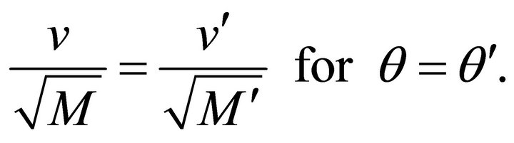
A simple approach of the two-body problem based on equivalent characterization of an orbit reveals some interesting new features that either were overlooked in the existing expositions [1-3], or did not appear at all. The relative motion can be characterized by a set of constants of motion in which the individual masses appear only through their sum. The conditions for various types of nesting or intersecting elliptic orbits of the individual gravitating particles are determined in a transparent way. Equivalent orbits, which by definition have the same semi-latus rectum and eccentricity, are realizable for different total masses provided the associated relative velocities are proportional to the square root of the total mass.
The origin of LVL vector [4-9] is highlighted through extracting from the eccentricity, which is a function in the energy and angular momentum reduced densities, and infinite set of vectors each of which provides the same information about the orbit. In passing, we mention that the LRL vector has an interesting history extending for more than three centuries [4,10,11,13-18], but because it was not well-known by physicists, it was rediscovered a number of times.
We finally derive a set of laws for equivalent orbits that relate their relative velocities, periods, areal velocities, and energies to the corresponding total mass. As far as we know, apart from the law of periods, these laws were not stated before.
In a subsequent work we show that the Galileo’s simple observations concerning the free fall cannot be elevated to a level of a principle, and highlight the contradiction between the predictions of the Newtonian mechanics and general relativity, with the former being not a true approximation to the latter.
2. Basics of Two-Body Central Force Problem
Consider a closed system of two particles of masses  interacting through a force that depends only on the separating distance r. We take our inertial frame the center of mass frame S and denote the relative position vector of
  with respect to
  by
by
 (2.1)
(2.1)
The relative velocity and acceleration are
 (2.2)
(2.2)
respectively (Figures 1 and 2). Since
 (2.3)
(2.3)
we have
 (2.4)
(2.4)
and the Newton’s second law of motion , where
  is the force acting on the first (second) particle, is automatically satisfied. From Equations (2.2ii) and (2.4ii) we have
 (2.5)
(2.5)
where 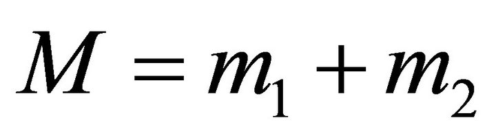 is the total mass of the system. Multiplying both sides with
  we obtain
 (2.6)
(2.6)
where
 (2.7)
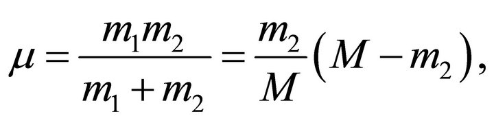
(2.7)
is the reduced mass of the system. It can be easily seen that, with M is fixed, the reduced mass is an increasing function in  with a minimum value
 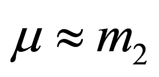 for
for 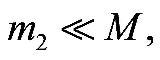 and a maximum value
  for
for  m1. The positions and velocities of the two particles satisfy relations similar to (2.5) and (2.6), namely
 (2.8i)
 (2.8ii)
From (2.6) we have
 (2.9)
(2.9)
where
 (2.10)
The relative momentum is defined by
 (2.11)
The Kinetic energy of the system is
 (2.12)
The work done by the internal forces on the particles when displaced by  respectively is
 (2.13)
The central force is derivable from the potential
 , (2.14)
and hence
 (2.15)
As a result  and the mechanical energy
  is conserved. Because
  the angular momentum about CM,
 (2.16)
is conserved at its initial value . It follows that the constant vector
  is always perpendicular to
 , and hence, both particles move in a plane through CM and perpendicular to
  Employing polar coordinates
  in the plane of motion with
  is the polar axis and
  is its unit vector, the equations of the relative motion (2.9) take the form
 (2.17)
where  denotes differentiation with respect to time. Equation (2.17ii) yields a first integral
 , which is a constant of motion. The available constants of motion:
 (2.18i)
 (2.18ii)
express the conservation of the total energy E and the angular momentum  respectively, where k is a unit vector perpendicular to the plane of motion.
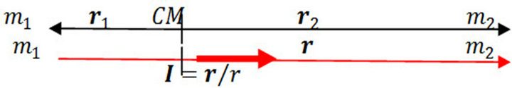
Figure 1. Position of m2 relative to m1 in CM system.

Figure 2. The relative acceleration for m1 > m2.
3. Motion under a Gravitational Force
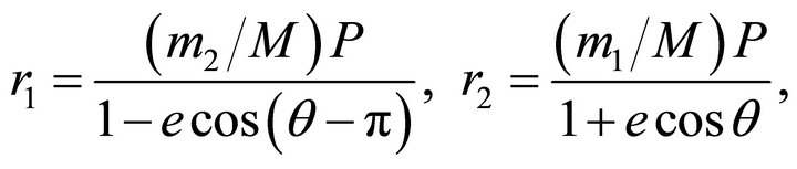
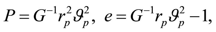
For the gravitational force 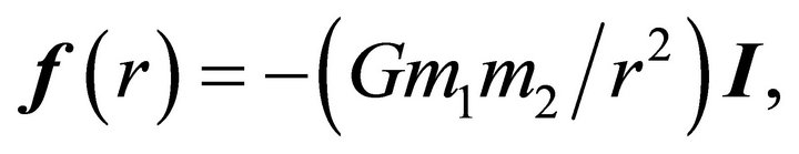 where G is the gravitational constant, the relative acceleration is, by (2.9),
 (3.1)
(3.1)
At an explicit discrepancy with Galileo’s law of free fall, which asserts that the acceleration of a freely falling particle in a gravitational field is independent of its mass, the latter form shows that the relative acceleration depends on the sum of the masses of the gravitating particles. Equations (3.1), in which the masses of the particles appear only through their sum, show that all characteristics of the relative orbit do not depend on how the total mass is divided between the two particles. However, the absolute acceleration of a particle, or its acceleration in the frame of the center of mass  depends only on the other particle’s mass as it is evident from (2.5) and (3.1). Indeed,
 (3.2)
(3.2)
Here, the constants of motion (2.18) take the forms
 (3.3)
(3.3)
 (3.4)
(3.4)
where we set in (2.18),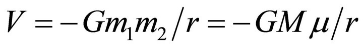 . The quantities
 ![]() and h represent the energy and angular momentum of the system per unit reduced mass; they will be called the reduced energy and angular momentum densities respectively.
and h represent the energy and angular momentum of the system per unit reduced mass; they will be called the reduced energy and angular momentum densities respectively.
The orbit of the system is determined by a well-known method [1-4],
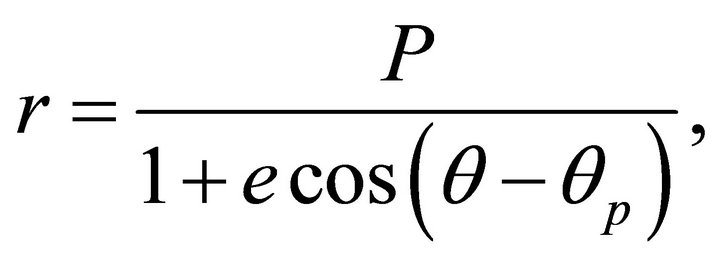 (3.5)
(3.5)
where  is a constant of integration that depends on the choice of the polar axis (i.e. the zero of
  it has nothing to do with the zero of time), and
 (3.6)
(3.6)
are the semi-latus rectum and the eccentricity of the orbit.
By a suitable choice of a new polar axis we may take  in (3.5), and by (2.8i) the orbits of the particles in
  are given by
 (3.7i)
where
 (3.7ii)
4. The Relative Orbit and Individual Orbits
The trajectory  of the system, or the relative orbit, can refer to the trajectory of either particle, say m2
  in a frame
  co-moving with
  and not rotating relative to the fixed stars, or in the frame S, in which case the measured length is
  and CM is the origin of the polar coordinates. The relative orbit in S in then the abstract locus
  with focus at the CM. This orbit is merely the collection of the pairs
  at various instants of time, referred to a polar system with origin at CM.
The relations (3.7) determine the orbits of the particles  and
and  in the center of mass’ frame
  It must be noted that
  in (3.7) refers to the polar angle of the radius vector
  relative to the polar axis
 , and it is also the polar angle of the radius vector
  with the polar axis
  which is directly opposite to the axis
 .
.
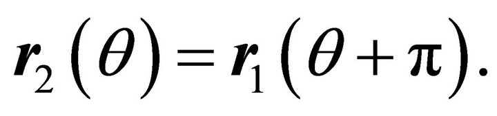
Assuming , the latter two relations show that each particle traces out an ellipse with the same eccentricity but with different semi-latus rectums, and the particles are radially opposite to each other with respect to one focus. In other words, each radius vector makes the same angle
  with the polar axis of the corresponding trajectory, with the polar axes of the two trajectories are directly opposite to each other. The two ellipses have one common focus at the center of mass, while the other foci are on two opposite sides on the polar axis
  (Figure 3). The case of
  is drawn in (Figure 4).
In one polar system of coordinates with polar axis , the simultaneous positions of the particles at their trajectories are expressed by the equations
 (4.1)
(4.1)
with  and
and  are the simultaneous polar angles of
  and
and  respectively. We note that while there is no restriction on
  for elliptic orbits,
  for parabolic orbits, and
  for hyperbolic orbits.
Because they have the same eccentricity e, the orbits of the system and its components (i.e.  and
and ) are
) are
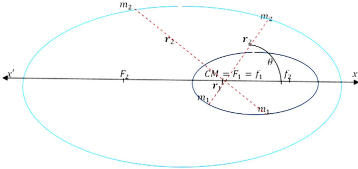
Figure 3. Nesting elliptical orbits.
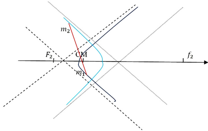
Figure 4. Unbound orbits always intersect.
the same type of conic sections. By (3.10ii) the orbit’s type is determined by the quantity
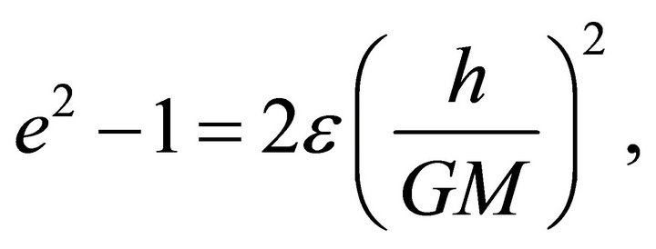 (4.2i)
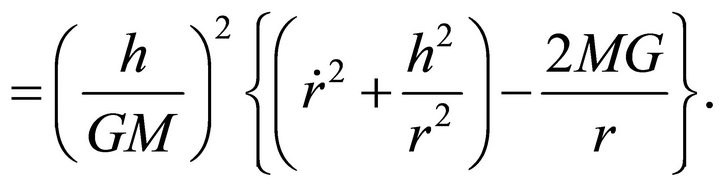 (4.2ii)
Depending on  (or E) the orbit is a hyperbola if
 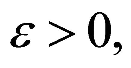 a parabola if
 , an ellipse if
 , or a circle if
  i.e.
i.e.  The knowledge of the relative orbit and the mass of each particle determines the orbit of each particle in S by (3.7). Conversely, if the trajectory of each particle is known in S, the system’s trajectory is determined by
 .
.
5. Intersection of the Particles’ Orbits
We determine here a necessary and sufficient condition for the intersection of the orbits of the two particles in the center of mass’ frame S. The intersection of the orbits can happen if and only if there exists a value of  for which
 (5.1)
(5.1)
If such a value exists then there exists another value, namely , which corresponds to another intersection, i.e.
  Substituting from (3.7) in (5.1) and solving for
  we obtain the equation
 (5.2)
(5.2)
in which  are known. This equation may or may not have solutions for
  The orbits intersect if the latter equation admits solutions; otherwise they do not.
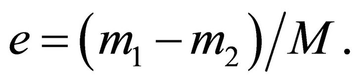
The special case  which corresponds to a circular motion, reduces (5.2) to the impossible for
  and to an identity in
  for
for  Thus, for
  the particles trace out circles with a common center; these circles do not intersect if the particles’ masses are different and coincide if they are equal (Figure 5).
We proceed now to consider the general case in which 
Necessary and Sufficient Condition for Intersection: As  Equation (5.2) yields
 (5.3)
(5.3)
which has solutions if and only if
 (5.4)
(5.4)
We distinguish the following cases 1) If (5.4) holds the two orbits interest at two points:
 (5.5)
(5.5)
This applies to all types of orbits, bound or unbound. For 
 and the radii vectors of the points of intersection are perpendicular to the polar axis.
2) For unbound motion the inequality (5.4) holds strictly, since , and we have always two distinct points of intersection (Figure 4). Because in this case the argument of the arccosine is strictly less than 1,
  cannot be a solution, and the orbits of unbound motion cannot be tangential.
3) There can be no intersection of orbits if  m2. The latter condition may hold only in bound motion (elliptic orbits), where
  In this case the orbit of the heavier particle lies entirely inside the orbit of the lighter one (Figure 3).
4) Assuming  Equation (5.3) admits the solution
  which corresponds to tangential orbits (Figure 6), if
 (5.6)
(5.6)
Since the value prescribed for e by the last equation is less than 1, tangential orbits can occur only in bound motion.
5) When the inequality (5.3) holds strictly (i.e. with (>)) there exist two intersections specified by (5.5) (Figures 4 and 7).
In the special case  the points of in-
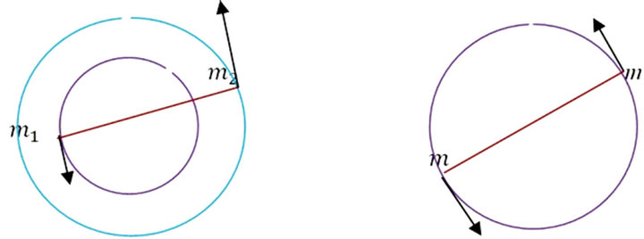
Figure 5. The case (e = 0) corresponds to concentric circles for m1 > m2 (left), and to one circle for m1 = m2 (right).
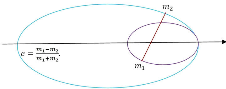
Figure 6. Orbits can be tangential only for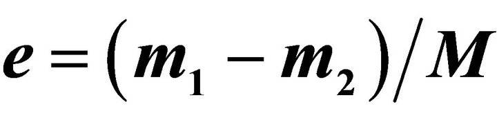 .
.
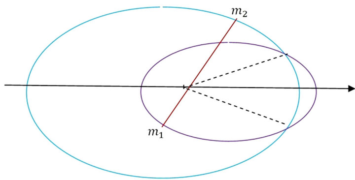
Figure 7. Intersecting elliptic orbits.
tersection occur for  i.e. when the radii vectors are perpendicular to the polar axis (Figure 8).
6) When the mass  is dominant
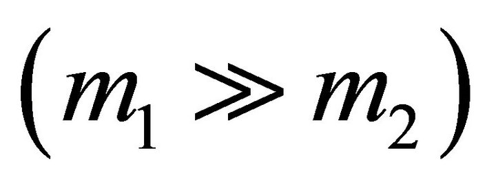 , the condition of intersection (5.4) cannot hold for bound motion. This implies that orbits in bound motion do not intersect if one mass is dominant. In this case the orbit of the lighter mass encircles the orbit of the heavier one. This persists for one dominant mass and many minor lighter masses whose mutual interactions can be neglected in comparison with the magnitude of their interaction with the dominant mass. In this case the orbit of each minor particle does not intersect the orbit of the dominant mass. An example of this is the solar system.
6. Orbit’s Characterization
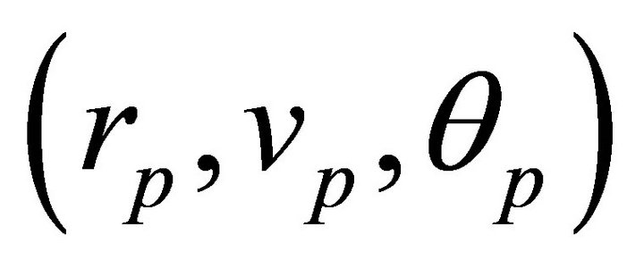
For simplicity we assume that the polar axis is chosen to pass through the perihelion, and hence  in (3.5). The orbit is then determined in the plane of motion by a set of two parameters
  which can also refer to any orbit in any plane of motion. i.e., we may look on one orbit as a representative of a class of equivalence of orbits, with two orbits are equivalent if they have the same eccentricity and semi-latus rectum. It is clear that the elements of the class of orbits
  result from one orbit through rotation, inversion, or translation. The latter fact follows from the homogeneity of the space with respect to any closed system and hence its isotropy [19].
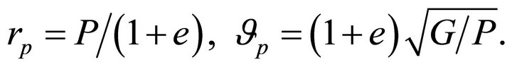
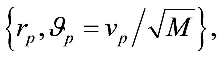
Equivalent Characterization: At an arbitrary point of the system’s trajectory, both components of the relative

Figure 8. The radii vectors at the intersections are perpendicular to the polar axis when m1 = m2.
velocity  in the moving system
  are non-zero in general. At the perihelion,
  , the radial velocity vanishes
  and the velocity is purely tangential; it is given by
  Inserting these values in (3.6i) and (4.2ii) yields
 (6.1)
(6.1)
 (6.2)
(6.2)
Assuming that the motion is in the positive sense and solving for  we get
 (6.3)
(6.3)
The characterization  is based on the 1-1 correspondence
 (6.4)
(6.4)
in which the first equation follows from (3.5), and the second from
 (6.5)
(6.5)
Equation (6.5) results from calculating e from (6.4i) and substituting for P from (6.1) in terms of  and
and .
.
We have found therefore the explicit forms of the 1-1 correspondences
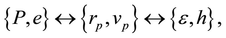 (6.6)
(6.6)
given by (6.3) and (6.4). The latter correspondences can also be obtained on noting that the Jacobian determinant in each case is not zero for the allowed range of variables. Excluding the pair  each pair obtained from the quantities
 (6.7)
(6.7)
is sufficient as any of the pairs (6.6) to determine the orbit. Moreover, given a pair the remaining pairs are determined uniquely.
Any trajectory  can be realized by
  given by (6.4i) and
 (6.8)
(6.8)
Since  any distance
  can be made a common perihelion for a family of trajectories simply by letting
  varies in the range
 (6.9)
(6.9)
According to the value  at
at  the following types or orbits occur:
• Circular Orbits: Setting  in (6.8) we find that a circular orbit is realized if
 (6.10)
• Elliptical orbits occur for  which by (6.8) is equivalent to:
 (6.11)
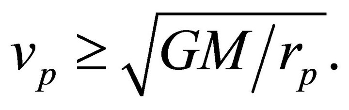
• A parabolic orbit occurs for , in which case (6.8) yields
 (6.12)
• Hyperbolic orbits occur for  which is equivalent to:
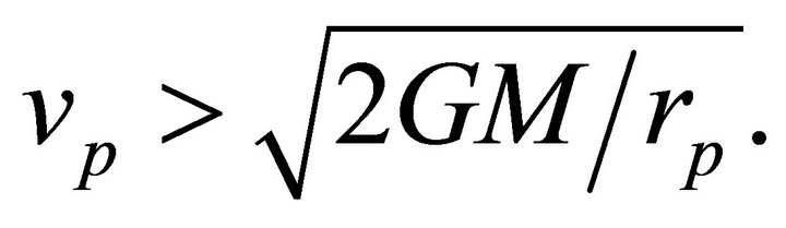 (6.13)
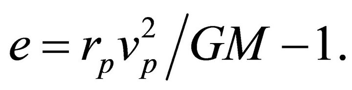
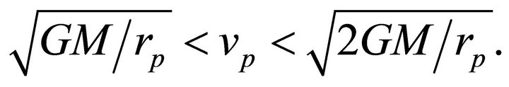
The Escape Velocity: The escape velocity is the minimum relative velocity at the perihelion which yields an unbound orbit; it is given by (6.12). Fixing  and
and  but changing the total mass slightly in the vicinity of the value
  can change the orbit from bound to unbound or vise-versa. This applies also to changing the mass of one body while keeping the other fixed.
Kepler’s Third Law: The period  of a bound motion is derived as usual [1-3]
 (6.14)
where a is the length of the semi-major axis of the ellipse.
7. The Laplace-Runge-Lenz Vector
The solutions of the equation of motion (3.1) contain six arbitrary constants which are determined by the initial conditions . Since any constant of motion
  is a function of the coordinates and velocities, there can be no more than five functionally independent constants of motion [20], because if there were six of them then the solution of the six equations
  for the coordinates and velocities yields them all constants, which means that there is no motion, or no force. For central motion, four constants of motion are already available, namely,
  (or L and E) which determine the plane of motion, the eccentricity, and the latus rectum of the orbit.
A given pair , (or
, (or ), determines a triple infinite family of orbits. These correspond to determine the plane of motion
  through CM by two parameters, which are the components of its unit normal (unit of angular momentum), and to determine the direction of the perihelion vector
  in
in  by one parameter, which is the angle
  it makes with the polar axis. Alternatively, an orbit is determined by the perihelion vector
  and the relative velocity vector
  in the plane
  perpendicular to the perihelion vector. However, with
  is given, the perihelion vector (or
 ) is determined in the 3-space by two parameters, say
 ; and with
  is given, the relative velocity vector (or
 ) is determined by one parameter in the plane
  Thus we need to fix five parameters, or initial conditions, to realize one specific orbit; the sixth initial condition corresponds to a zero radial component of the relative velocity at the perihelion. In our previous treatment, an orbit
  (or equivalently
 ) refers to that in the given plane of motion and passing through the given perihelion
  Without specifying
  we still have a one parameter family of equivalent orbits
  in the plane of motion, enveloped by a circle of radius
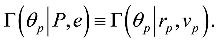
  which is formed by their perihelions. It is understood that the parameters that follow (|) are held constant.
If we restrict our discussion to the plane of motion then only four initial conditions 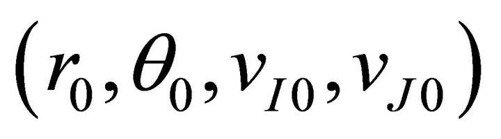 are involved, and only three parameters, say
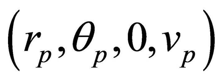 , are necessary to determine the orbit. To set up the link between the three parameters necessary to determine an orbit and the constants of motion we revert to the 1-1 correspondences (6.6) which are valid for a fixed M. Because of these correspondences, the same one-parameter family of orbits
  determined by
or  is also determined by
  i.e.
i.e. 
 This means that even knowing the energy and the angular momentum vector does not determine the orientation of the orbit in the plane of motion, and that any additional independent constant of motion can only specify the axis of symmetry of the orbit, or
  We shall see now that the Laplace-Runge-Lenz vector [4-9] plays the role mentioned in the latter statement, and moreover, there exist an infinite set of LRL vectors.
To see how the familiar LRL vector emerges we consider the equality
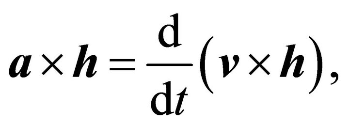 (7.1)
(7.1)
which is valid for any central force since 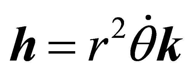 is conserved. As long as the force of interaction obeys the inverse square law we have
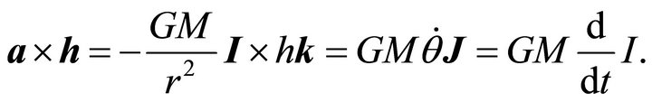 (7.2)
(7.2)
Comparing the latter two expressions we obtain
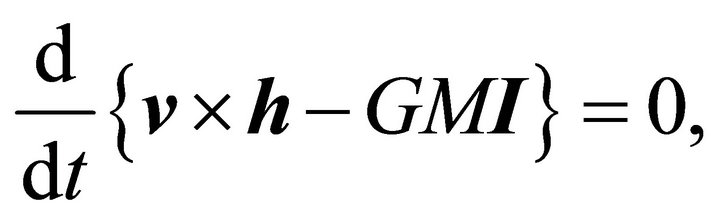 (7.3)
(7.3)
which means that the vector field
 (7.4)
(7.4)
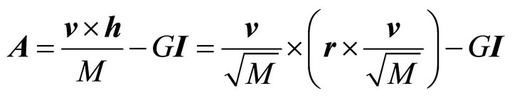
defined on every orbit, is constant on each orbit; it is called the LRL vector.
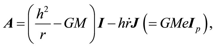
Another LRL vector can be obtained from the inverse square law (3.1):
 (7.5)
(7.5)
which shows that the vector field
 (7.6)
(7.6)
is also a constant of motion.
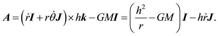
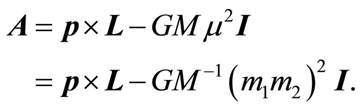
For the time being we adhere to the familiar LRL vector A. It is clear that the vector A is perpendicular to L, and thus is in the plane of motion . The analytic expression of this vector is
 (7.7)
(7.7)
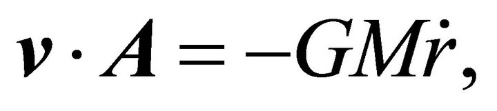
Taking the inner product of A and v, we obtain
 (7.8)
(7.8)
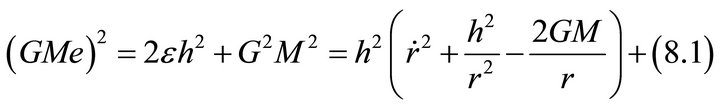
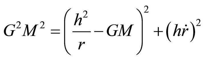
which shows that the vector A is perpendicular to the velocity (and to the orbit) only at the perihelion. The length of LRL vector,
 (7.9)
(7.9)
depends on the system’s energy and angular momentum reduced densities. By the first equality in (6.2), 
 and hence
 (7.10)
The vector A which is constant on an orbit has the same value it takes at the perihelion of that orbit:
 (7.11)
where  is the value I at the perihelion, i.e.
  . We could have obtained the latter relation from (7.7) through setting the second term equal to zero at the perihelion and employing (6.5):
  The vector A doesn’t exist for
  and when exists
 , it is parallel to the perihelion vector.
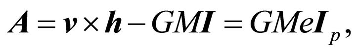
The familiar definition of LRL vector is obtained by multiplying the right-hand side of (7.4) by :
:
 (7.10)
This vector is constant at the value
 For
For ,
,
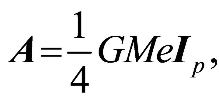 and when m1 is dominant, i.e.,
  we get the commonly used form of LRL vector:
 (7.11)
The utility of the LRL vector in determining the orbit’s orientation comes from the local information it provides. i.e., any observations of  and
and  and consequently
  are sufficient to determine the perihelion (and the orbit). If the calculated value of A is along a unit vector
  then starting from the focus CM we know in which direction the perihelion exists and where. For a given h the motion takes place in the plane
  that contains the CM and is perpendicular to h; A is along the perihelion vector in this plane. Moreover, and since e is expressible in terms of
 , the only new information that A provides and not provided by h and
 ![]() is contained in
is contained in , which is determined by the angle
  it makes with the polar axis. To see how
  injects this new information in an orbit, we first determine the relation between the coordinates of a point of an orbit on which the vector field
  takes the value
  The radial component of
  is on one hand the spherically symmetric field
 (7.12)
and on the other hand
 (7.13)
Equating these two expressions yields
 (7.14)
which is a surface of revolution spanned by all orbits  that have the same perihelion vector
 ; it is an ellipsoid of revolution if
 , a paraboloid of revolution if
 , and a hyperboloid of revolution if
  If h is known, the orbit is determined by the intersection of the surface (7.14) and the plane of motion. Thus the constants of motion h and A determine a unique orbit
 (7.14)
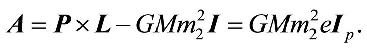
Conversely, we prove here that the LRL vector field is implied by the orbital motion, which endows it with one value on each possible orbit. Let  be the value of I at the perihelion. The LRL vector is obtained through the following implications resulting from the orbit equation (7.15)


Thus, the vector A is constant on an orbit (7.15) at its value at the perihelion, namely 
The latter results can be rephrased as follows: provided the system total mass is fixed and the plane of motion is given, there corresponds to each orbit  a unique value
 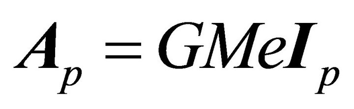 of the LRL vector A. And conversely, there corresponds to each value
  of A a unique orbit with
  pointing in the direction of its symmetry.
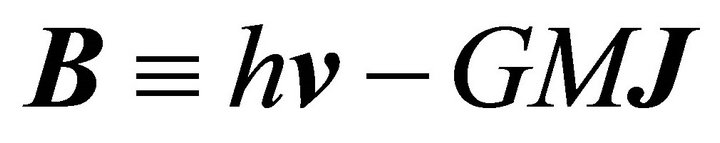
8. An Infinite Set of LRL Vectors
Any unit vector  can be chosen as the axis of symmetry of an orbit
  The mystery of LRL vector is resolved if we can derive from
  a vector constant of motion. This can be achieved if e can be expressed as a norm of a vector function in the coordinates and velocity components, and possibly in some constants of motion. The Equation (4.2i) (or (7.9)) written in the form:
provides the clue. The constant of motion on the furthest right-hand side is a function of the constants of motion  It is clear that each of the vectors
 (8.2a)
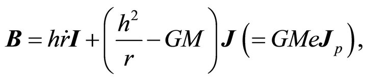 (8.2b)
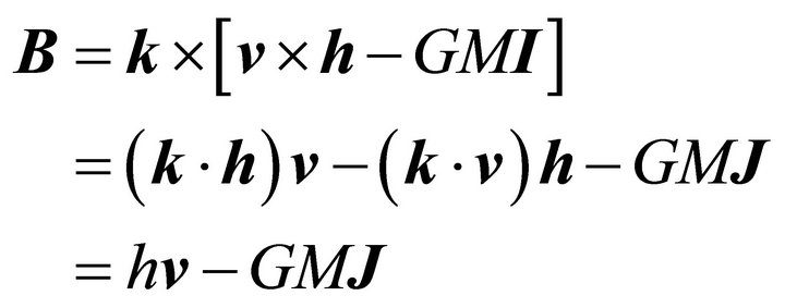
fulfills our quest, and is a constant of motion. The constancy of A was already proven, while the constancy of B follows from the fact,
 (8.3)
(8.3)
The vector B is constant at the value 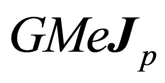 which it takes at the perihelion
 . Other possible factorizations of e, which are not just different by a sign from the given ones, are not constants of motion. By (8.2) the vectors A and B preserve their forms under rotations or translations; a fact which promotes a search for a coordinate independent expressions for A and B. Indeed,
 (8.4)
(8.4)
and the vector A, which is a constant of motion at an orbit, is of covariant form under rotation, inversion, and translation. The covariant expression for B is
 (8.5)
(8.5)
Since  the only information B adds to that given by
  is contained in
  the directrix of the orbit is along
  which is perpendicular to the perihelion vector. Indeed,
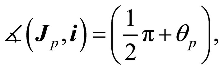 and B indicates that the directrix is at this angle with the polar axis, or the perihelion vector is at an angle
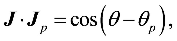
  with the polar axis. We may arrive to the same result through taking the inner product of J by both expressions of B on the claimed orbit:
and

Equating these expressions we get the same orbit (7.14).
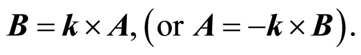
Starting from A and B we may construct an infinite set of LRL vectors, with each vector has a meaning similar to that of A. Indeed, any vector of the form  where
where  is constant on an orbit
 at the value
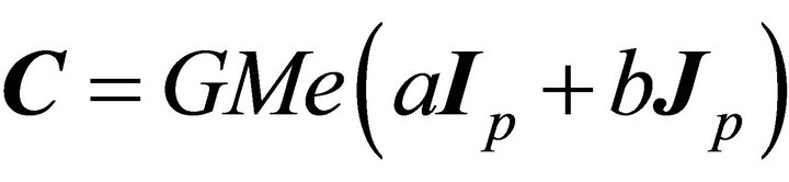 . Without loss of generality we take
 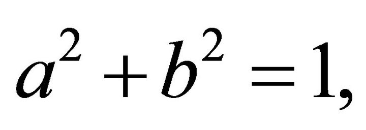 and set
 ![]()
![]() ,
, 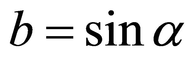 , where
  is the angle that C makes with A, i.e., C results from A through a rotation by an angle
  Noting that

we get

which yield the same orbit (7.15). This result could be foreseen through the equivalence
It is clear that 
Starting from A alone we may construct an infinite set of LRL vectors each of which plays the same role as A. If O is an arbitrary orthogonal  matrix, then each vector
 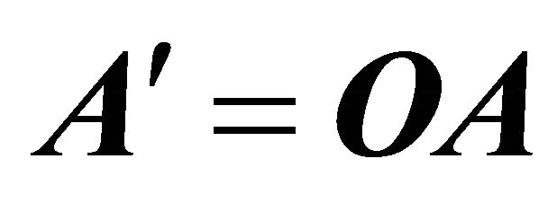 is a constant of motion
 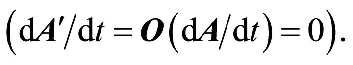 The equivalence,
 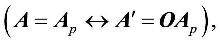 shows that the same information concerning the orientation of an orbit is contained in an LRL vector as in its transforms. In particular the vectors B and C result from A through rotations by
  and
and  respectively.
9. Equivalent Orbits
We have already seen that given the plane of motion, (or given ), the pair
  determines an 1-parameter family of equivalent orbits
 , enveloped by a circle
  in the plane of motion. It is understood that all quantities which succeed the vertical bar are held as constant parameters, whereas
  is a free parameter whose values distinguish between the members of this family. Letting
  vary we obtain a 3- family of equivalent orbits
  enveloped by the spherical surface
Given  and the perihelion vector
  in the 3- space there exists a 1-parameter family of equivalent orbits
  with the rotation angle
  about
about  is the family parameter. This 1-family generates a conic section of revolution
  given by (7.14), which is perpendicular to the perihelion vector at its vertex.
Letting the direction of the perihelion vector arbitrary gives a 3-parameters family of equivalent orbits  , which generates a 2-parameter family of conic sections of revolution
  enveloped by a sphere of radius
  It is clear that the family of equivalent orbits
  results from one orbit
  under the action of orthogonal transformations
 (9.1)
(9.1)
where O is an arbitrary orthogonal  matrix and b is an arbitrary
  vector [21]. Indeed, and because the space is homogeneous with respect to a closed two-body system, the latter remains equivalent to itself after a rotation, translation or inversion applied to it as a whole. Mathematically, it sufficient to note that the characteristics of an orbit
  are invariant, since the norm of a vector is preserved under (9.1), while the vector
  is mapped to
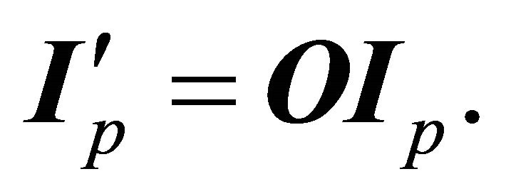
If we let 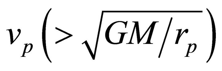 vary we obtain 4-parmaeter family of orbits
  enveloped by the sphere
 , with each point
  of the enveloping sphere is the vertex of a 1-parameter family of solid conic sections
 , or equivalently, the vertex of a 2-parameter family
  of orbits. Each value of
  corresponds to 1-family of equivalent orbits, and orbits belonging to different 1-families (i.e. different
 ) are non-equivalent. When moving from a family to another the curvature decreases as
  increases, and orbits are more flattened with increasing
  The family with
  is subtended by all other families. As
  increases the orbits gets broader and longer but remain bound till reaching the escape velocity, at which the orbits become unbound. Letting
  vary, each point
  of the space (excluding CM) is a vertex of a 2-parameter family of orbits
It is noted that the LRL vector changes with  though
  is fixed; this is because
  and h changes, and hence e. Throughout our previous discussion the total mass M was fixed. We shall see soon that equivalent orbits with different velocities can be realized, however, with different total masses.
10. Laws of Equivalent Orbits
With M is fixed, equivalent orbits are characterized by the same  Although a given orbit has specific values of angular momentum and energy reduced densities, there correspond to the same orbit different angular momentum
  and energy
  depending on the distribution of the total mass M among the two particles. Thus the angular momentum and energy associated with the same relative orbit (and fixed M) may vary in absolute value from infinitesimal values corresponding to an infinitesimal reduced mass
  to maximum values
 and
and  corresponding to
We seek here a mass-independent characterization of relative orbits. Setting
 (10.1)
the relations (6.1) and (6.5) yield  in terms of
  and
and  by
by
 (10.2)
provided  Conversely, a given orbit
  corresponds to
 (10.3)
It follows from (10.2)-(10.3) that equivalent orbits  are also characterized by the pair
 (10.4)
which embodies what we may call “degeneracy”, where the same orbit 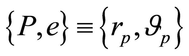 can be realized by multiple values of
  and M. The LRL vector
 (10.5)
is constant, on an orbit with perihelion vector  at the value
  which is independent of the total mass. The form (10.5) is thus a mass-independent characterization of equivalent orbits (10.4).
The following laws govern equivalent orbits with different total masses:
1) Given  and
and , the same orbit occurs for any
  provided the corresponding
  leaves
  unchanged. Quantitatively, the same orbit occurs with a new mass
  provided the new relative velocity is
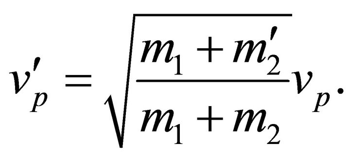 (10.6)
2) No matter how a fixed total mass M is distributed between the two particles, the same relative trajectory occurs for the same initial conditions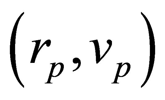 .
.
3) Law of Periods: by (6.14), systems with identical bound trajectories have periods that are inversely proportional to the square root of their total masses
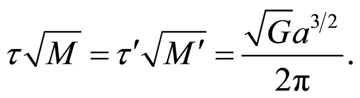 (10.7)
If Jupiter, whose mass is about 1000 times the earth’s mass, replaces the earth on its orbit then its period will be about four hours less than our year.
Defining
 (10.8)
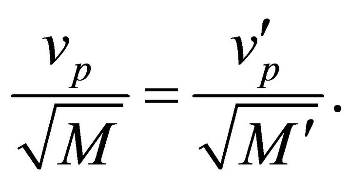
and employing (6.3) we obtain
 (10.9)
which shows that  is a characterization of equivalent orbits on equal footing with
  or
or . For equivalent orbits with different total masses M and M' we have
 , and hence 4) The Law of Areal Velocity:
 (10.10)
5) The Law of Orbit’s Energy
 (10.11)
But since  we have
 (10.12)
Combining the latter law with the Newton law of gravitation we obtain  at each point of the orbit. This relation however is not independent of the law of force and (10.12).
6) The Law of Angular Velocity: Two systems of total masses  and
and  can have equivalent trajectories provided they have the same
  and their respective relative velocities are proportional to the square root of their total masses:
 (10.13)
Denote the points of two equivalent orbits  corresponding to total masses M and M' by
  and
and  respectively, and take
  For
For  we have
  and by (10.10),
 (10.14)
7) The Law of Velocities: The relative velocities associated with the two orbits are
 (10.15)
The parenthesized quantities in the latter two equations are equal in magnitude for , because
  and
and . It follows that
  for
for  Multiplying the latter equation side to side by equation (10.14) yields
 (10.16)
The latter equation states that the relative velocity of the system is proportional to the square root of its mass. In other words, if the total mass M were replaced by  then its new velocity
  would be related to it its old velocity v at each point by (10.16).
8) System’s and Parts’ Angular Momenta: We derive here the relation between the magnitude of the total angular momentum  and the magnitudes of the angular momenta of its parts. This law is valid for any type of central force. From their definition (2.16) and from the fact that
 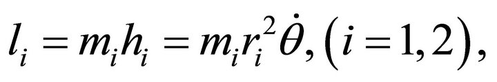 we have
 (10.17)
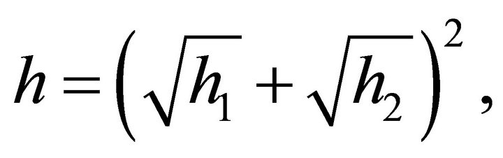
which is the law that determines the system’s areal velocity in terms of the areal velocities of its parts. From (10.17) we find that the magnitude of the total angular momentum given by
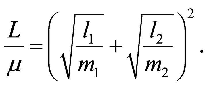 (10.18)
11. Conclusion
The approach followed in this work revealed features of the two-body problem that neither were highlighted in earlier expositions, nor appeared at all. Indeed, it was shown that the characteristics of the system’s motion depend on its total mass, while those of the individual motions depend on the individual masses. The possible energies associated with equivalent orbits with the same mass vary in absolute value from an infinitesimal to a maximum value although the reduced energy and angular momentum densities are the same. The types of intersection or nesting of individual orbits were presented in a simple and a transparent manner. Corresponding to the infinite possible referential ways of specifying the absolute rotational positioning of a two-body system, an infinite set of LRL vectors can be constructed, all fixing a unique orientation of the orbit with respect to the remote universe. The commonly used LRL vector is an approximation of one of the vectors derived in our approach. As far as we know, and apart from the law of periods, the laws of equivalent orbits we have derived, which included the laws of periods, areal velocities, angular velocities, velocities, total angular momentum, were never considered before. The latter laws, together with other features of the two-body motion contradicting the general relativistic description will be the subject of a forthcoming work.
REFERENCES
- H. Goldstein, C. P. Poole and J. L. Safko, “Classical Mechanics,” Addison Wesley, Boston, 2001.
- S. W. Groesberg, “Advanced Mechanics,” John Wiley & Sons, Inc., Hoboken, 1998.
- S. R. Spiegel, “Theoretical Mechanics,” In: Schaum Outline Series, Mc Graw Hill Book Company, New York, 1967.
- H. Goldstein, “More on the Prehistory of the Runge-Lenz Vector,” American Journal of Physics, Vol. 44, No. 11, 1976, pp. 1123-1124. doi:10.1119/1.10202
- A. Alemi, “Laplace-Runge-Lenz Vector,” 2009. www.cds.Caltech.edu/Wiki/Alemicds205final.pdf
- “Laplace-Runge-Lenz Vector,” Wikipedia, 2013. http://en.wikipedia.org/wiki/Laplace%E2%80%93Runge%E2%80%93Lenz_vector
- P. G. L. Leach and G. P. Flessas, “Generalizations of the Laplace-Runge-Lenz Vector,” Journal of Nonlinear Mathematical Physics, Vol. 10, No. 3, 2003, p. 340.
- J. Moser, “Regularization of Kepler’s Problem and the Averaging Method on a Manifold,” Communications on Pure and Applied Mathematics, Vol. 23, No. 4, 1970, pp. 609-636. doi:10.1002/cpa.3160230406
- H. H. Rogers, “Symmetry Transformations of the Classical Kepler Problem,” Journal of Mathematical Physics, Vol. 14, No. 8, 1973, p. 1125. doi:10.1063/1.1666448
- W. R. Hamilton, “The Hodograph or a New Method of Expressing in Symbolic Language the Newtonian Law of Attraction,” Proceedings of the Royal Irish Academy, Vol. 3, 1847, pp. 344-353.
- W. R. Hamilton, “Applications of Quaternions to Some Dynamical Questions,” Proceedings of the Royal Irish Academy, Vol. 3, 1847, Appendix III.
- J. Hermann, “Unknown Title,” Giornale de Letterati D’ Italia, Vol. 2, 1710, pp. 447-467.
- J. Hermann, “Extrait d’une lettre de M. Herman a’ M datée de Padoüe le 12, Juillet 1710,” Histoire Toire de l’Academie Royale des Sciences (Paris), 1732, pp. 519- 521.
- J. Bernoulli, “Extrait de la Response de M. Bernoulli a M. Herman date de Basle le 7. October 1710,” Histoire de l’Academie Royale des Sciences (Paris), 1732, pp 521- 544.
- P. S. Laplace, “Traite de Mecanique Celeste,” Tome I, Premiere Partie, Liver II, 1799, p. 165.
- J. W. Gibbs, J. W. Gibbs and E. B. Wilson, “Vector Analysis,” Scribners, New York, 1910, p. 135.
- C. Runge, “Vektoranalysis,” Verlag Von S. Hirzel, Leipzig, 1919.
- W. Lenz, “Uber den Bewegungsverlauf und QuantenzustAnde der Gestorten Keplerbewegung,” Zeitschrift fur Physik, Vol. 24, No. 1, 1924, pp. 197-207. doi:10.1007/BF01327245
- W. Rindler, “Essential Relaivity,” Springr-Verlag, Berlin, 2006.
- N. W. Evans, “Superintegrability in Classical Mechanics,” Physical Review A, Vol. 41, No. 10, 1990, pp. 5666- 5676. doi:10.1103/PhysRevA.41.5666
- F. D. Lawden, “Tensor Calculus and Relativity,” Chapman and Hall, London, 1975.