Applied Mathematics
Vol. 3 No. 11 (2012) , Article ID: 24377 , 7 pages DOI:10.4236/am.2012.311222
Limit Theorems for a Storage Process with a Random Release Rule
Department of Mathematics, Faculty of Science, King Abdulaziz University, Jeddah, Saudi Arabia
Email: mezianilakhdar@hotmail.com
Received August 29, 2012; revised October 8, 2012; accepted October 15, 2012
Keywords: Storage Process; Random Walk; Strong Law of Large Numbers; Central Limit Theorem
ABSTRACT
We consider a discrete time Storage Process  with a simple random walk input
  and a random release rule given by a family
  of random variables whose probability laws
  form a convolution semigroup of measures, that is,
  The process
  obeys the equation:
 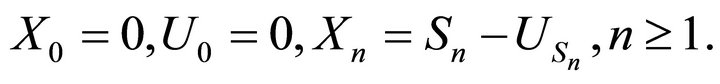 Under mild assumptions, we prove that the processes
  and
and  are simple random walks and derive a SLLN and a CLT for each of them.
1. Introduction and Assumptions
The formal structure of a general storage process displays two main parts: the input process and the release rule. The input process, mostly a compound Poisson process , describes the material entering in the system during the interval
 . The release rule is usually given by a function
  representing the rate at which material flows out of the system when its content is
 . So the state
  of the system at time
  obeys the well known equation:
 .
.
Limit theorems and approximation results have been obtained for the process  by several authors, see [1-5] and the references therein. In this paper we study a discrete time new storage process with a simple random walk input
  and a random release rule given by a family of random variables
  where
where  has to be interpreted as the amount of material removed when the state of the system is
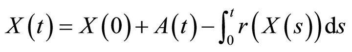
  Hence the evolution of the system obeys the following equation:
 where
where ,
,  for i.i.d. positive random variables
  with
with  and
and 
We will make the following assumptions:
1.1. The probability distributions  of the random variables
  form a convolution semigroup of measures:
 , (1.1)
We will assume that for each ,
,  is supported by the interval
  that is,
  Consequently, for
  the distribution of
  is the same as that of
 , (see 2.2
 ).
).
1.2. Also we will need some smoothness properties for the stochastic process  These will be achieved if we impose the following continuity condition:
 (1.2)
(1.2)
where  is the unit mass at 0 and the limit is in the sense of the weak convergence of measures.
1.3. The two families of random variables  and
and  are independent.
2. Construction of the Processes  and
and 
2.1. Let  be a probability measure on the Borel sets
  of the positive real line
  and form the infinite product space
 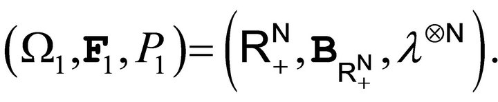 Now, as usual define random variables
  on
on  by:
by:
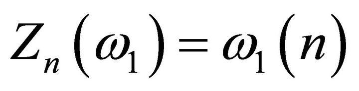 , if
, if 
Then the  are independent identically distributed with common distribution
  We will assume that
  and
and 
2.2. Let  be a semigroup of convolution of probability measures on
  with
with  and satisfying (1.2) then, it is well known, that there is a probability space
  and a family
  of positive random variables defined on this space such that the following properties hold:
 . Under
  the distribution of
  is
is ,
, 
 . For
. For , the random variables
  and
and  have under
  the same distribution
 . For every
  the increments
  are independent.
 . For almost all
  the function
 is right continuous with left hand limit (cadlag).
From  we deduce:
 . The function
  is measurable on the product space
2.3. The basic probability space for the storage process  will be the product
  Then we define
  by the following recipe:
 (2.3)
(2.3)
 if
if 
 where
where  is the simple random walk with:

2.4. Since  is a simple random walk, the random variables
  and
and  have the same distribution for
 .
.
3. The Main Results
The main objective is to establish limit theorems for the processes  and
and . Since the behavior of
  is well understood, we will focus attention on the structure of the process
 . The outstanding fact is that
  itself is a simple random walk. First we need some preparation.
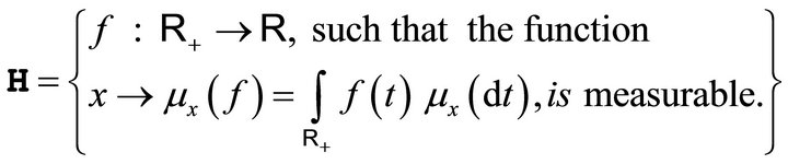
3.1. Proposition: For every measurable bounded function , the function
 is measurable. Thus for any Borel set
  of
of  the function
  is measurable.
Proof: Assume first  continuous and bounded, then from (1.2) we have
Now by (1.1) we have
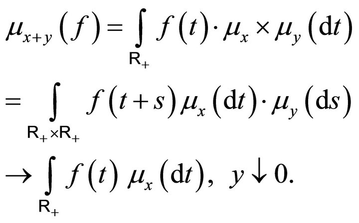
by (1.2) and the bounded convergence theorem. Consequently the function 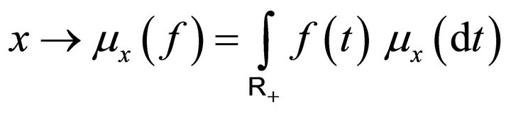 is right continuous for all
  hence it is measurable if
  is continuous and bounded. Next consider the class of functions:
then  is a vector space satisfying the conditions of Theorem I,T20 in [6]. Moreover, by what just proved,
  contains the continuous bounded functions
  therefore
  contains every measurable bounded function
  ■
■
3.2. Remark: Let , be the expectation operators with respect to
  respectively. Since
  we have
 , by Fubini theorem. ■
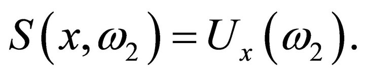
3.3. Proposition: Let  be a positive random variable on
  with probability distribution
  Then the function
  defined on
  by:
by:
 (3.3)
(3.3)
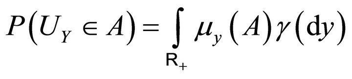
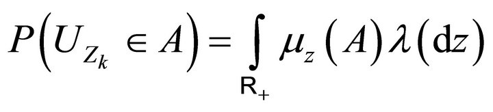
is a random variable such that
for every measurable positive function . In particular the probability distribution of
  is given by:
 (3.5)
(3.5)
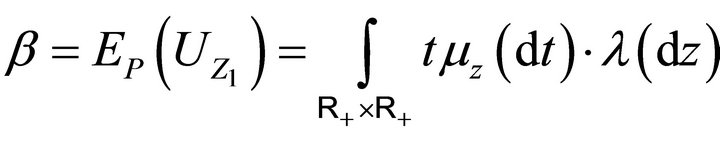
and its expectation is equal to
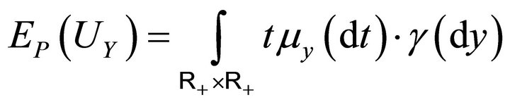 (3.6)
(3.6)
Proof: Define 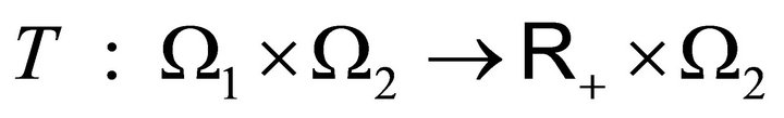 by
by
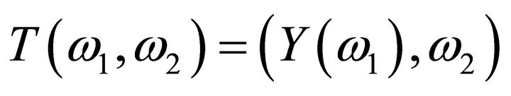 and
and 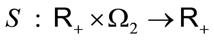 by
by
 It is clear that
  is measurable. Also
  is measurable by 2.2
  so
so  is measurable.
(3.4) is a simple change of variable formula since  ■
■
3.7. Proposition: For all , the random variables
 have the same probability distribution.
Proof: It is enough to show that for every positive measurable function , we have:
 (3.4)
(3.4)
Since  we can write:
But for each fixed  we get from 2.2
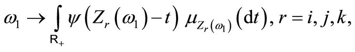
Applying  to both sides of this formula we get the first equality of (3.7). To get the second one, observe that the function
  is measurable (Proposition 3.1) and use the fact that under
 , the random variables
  and
and  have the same probability distribution by 2.4. ■
3.8. Theorem: The process  is a simple random walk with:
and 
Proof: We prove that for all integers  and all positive measurable functions
  we have:
 (3.8)
(3.8)
Let  be fixed in
 . By 2.2
  under
under  the random variables
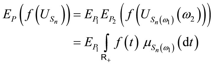
are independent. Therefore, applying first  in the L.H.S of (3.8), we get the formula:
 (*)
(*)
But  have distributions
 ,
,  , respectively. Thus:
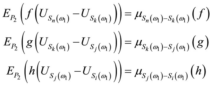
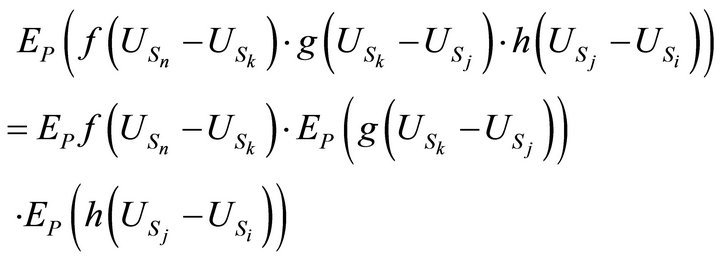
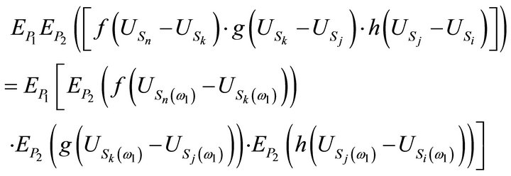
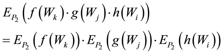
By Proposition 3.1, the R.H.S of these equalities are random variables of , independent under
  since they are measurable functions of the independent random variables
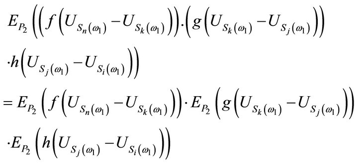
 Therefore, applying
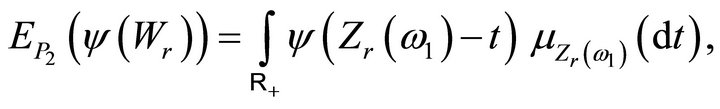
  to both sides of formula (*) we get the proof of (3.8):
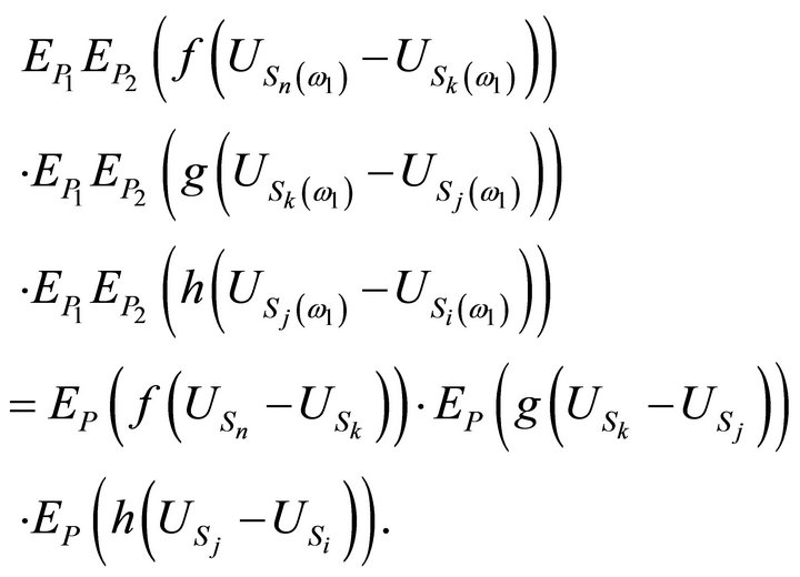
To achieve the proof, write  as follows:
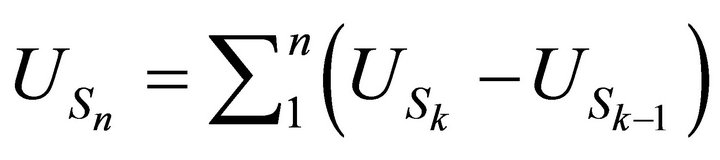 , where the
  are independent with the same distribution given by
according to (3.5). ■
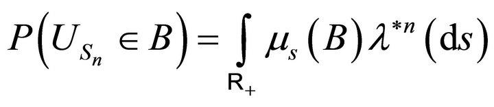
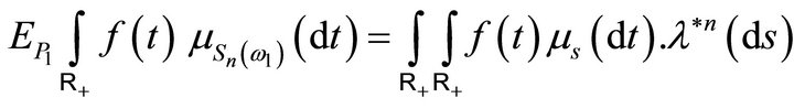
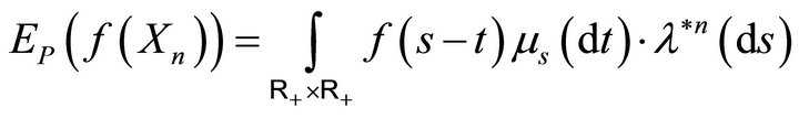
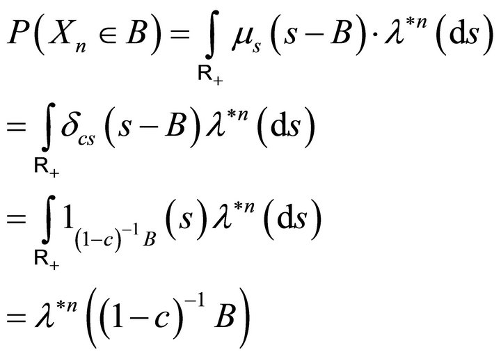
3.9. Proposition: For every positive measurable function , we have:
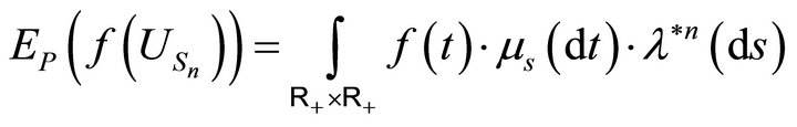 (3.9)
(3.9)
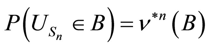
 being the n-fold convolution of the probability
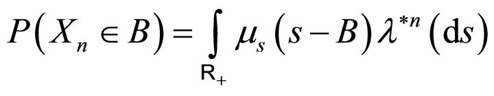
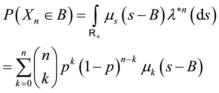
  In particular the distribution law of the process
  is given by:
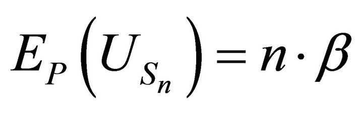
and its expectation is:
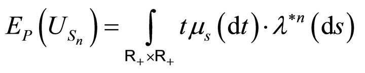
Proof: We have:
and, by Proposition 3.1, the function
 is a measurable function of
 . Since
  is a simple random walk with the
  having distribution
  the random variable
  has the distribution
 . So, by a simple change of variable we get:
 . So formula (3.9) is proved. To get the distribution law of the process
 , take
  equal to the characteristic function of some Borel set B. ■
3.10. Remark: Let  be the distribution of
 that is
 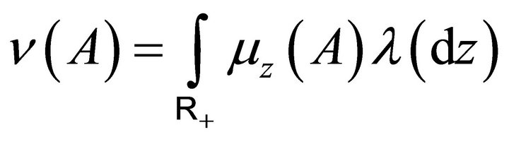 and let
 , then as a direct consequence of theorem 3.8,
 ■
■
Now we turn to the structure of the process . We need the following technical lemma:
3.11. Lemma: For every Borel positive function
 , the function
is measurable.
Proof: Start with , the characteristic function of the measurable rectangle
 , in which case we have
  Since by proposition 3.1, the function
  is measurable we deduce that
  is measurable in this case. Next consider the family
It is easy to check that  is a monotone class closed under finite disjoint unions. Since it contains the measurable rectangles, we deduce that
  Finally consider the following class of Borel positive functions
It is clear that  is closed under addition and, by the step above, it contains the simple Borel positive functions. By the monotone convergence theorem,
  is exactly the class of all Borel positive functions. ■
3.12. Theorem: The random variables  are independent with the same distribution given by: for
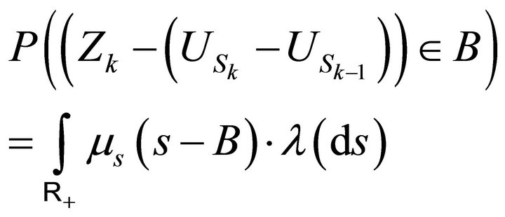 (3.12)
Consequently the storage process
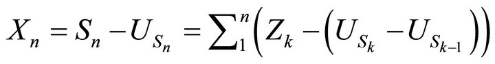 , is a simple random walk with the basic distribution (3.12).
Proof: For each integer , and each
  put:
put:
So it is enough to prove that for all  and all Borel positive functions
 , we have:
 (3.13)
From the construction of the process  we know that for
  fixed, the random variables
 are independent under
  (see 2.2 (iii)). So, applying
  to
to , we get:
 (3.14)
Now, since under , the distribution of
 is the same as that of
 , we have for each Borel positive function
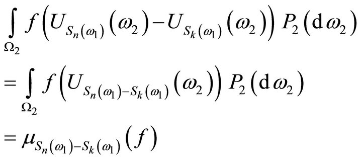
From lemma 3.11, the functions
 are Borel functions of the random variables
 , thus they are independent under the probability
  Therefore, applying
  to both sides of (3.14) we get (3.13). ■
As for the process , the counterpart of proposition 3.9 is the following:
3.15. Proposition: If  is positive measurable and if
 , then we have:
For the proof, use the formula  and routine integration.
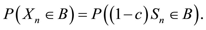
3.16. Example: Let  and let us take as measure
  the unit mass at the point
 , that is, the Dirac measure
 . It easy to check that
  for all
  in
in  Then for every probability measure
  on
on 
we have: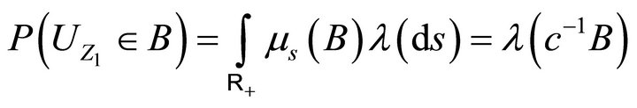 . This gives the distribution of the release process in this case:
Since we have , we deduce that the release rule consists in removing from
  the quantity
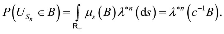
Likewise it is straightforward, from Proposition 3.14, that
from which we deduce that the distribution of the storage process is
One can give more examples in this way by choosing the distribution  or/and the semigoup
 . Consider the following simple example:
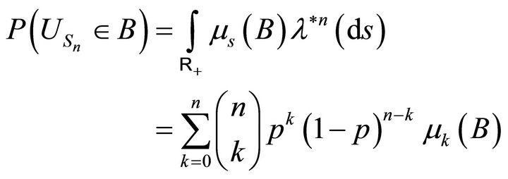
3.17. Example: Take  the 0 - 1 Bernoulli distribution with probability of success
  In this case the semigroup
  is a sequence
  of probabilities with
  supported by
  for
for  and
and  is the Binomial distribution. So we get from proposition 3.9
Likewise we get the distribution of  from proposition 3.15 as :
 . ■
. ■
4. Limit Theorems
Due to the simple structure of the processes  and
and  (Theorems 3.8, 3.12), it is not difficult to establish a SLLN and a CLT for them.
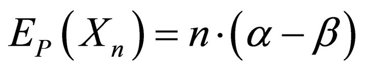
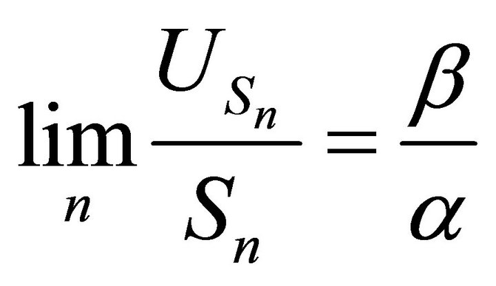
4.1. Theorem: For the storage process  and the release rule process
 , we have:
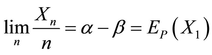
and
Proof: Since  and
and  are simple random walks with
  and
and  we have:
 and
and , by the classical S.L.L.N.
So we deduce:
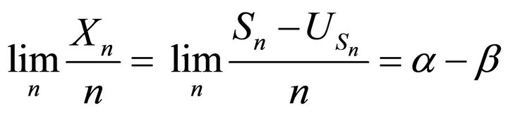
and

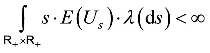
4.2. Proposition: Under the conditions:
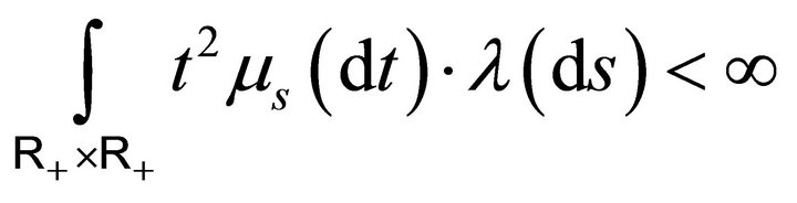 and
and
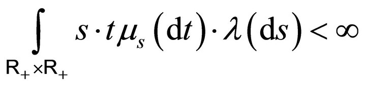 , the variances
  and
and 
of the random variables  and
and  are finite. The conditions can respectively be written as
and
 .
.
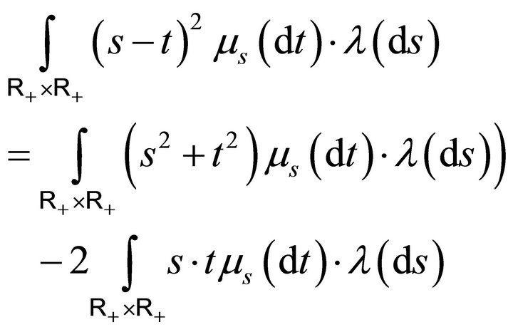
Proof: We have
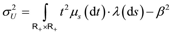 , so the first condition gives
 . On the other hand we have
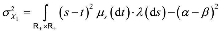
and
Since the variance  of
of  is finite we have
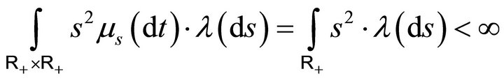 , so the conclusion follows. ■
Finally we get under the conditions of proposition 4.2:
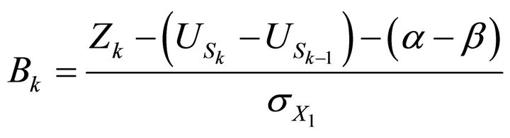
4.3. Theorem: Assume the conditions of proposition 4.2. Then the normalized sequences of random variables:
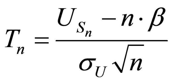 and
and 
both converge in distribution to the Normal law 
Proof: The condition of the theorem insures the finiteness of the variances  and
and  Now the conclusion results from the fact that
  and
and  are simple random walks and the Lindberg Central Limit Theorem. To see this, we use the method of characteristic functions. Let us denote by
  the characteristic function of the random variable
 . Since by Theorem 3.8 the components
  of
of  have the same distribution as
 , we have
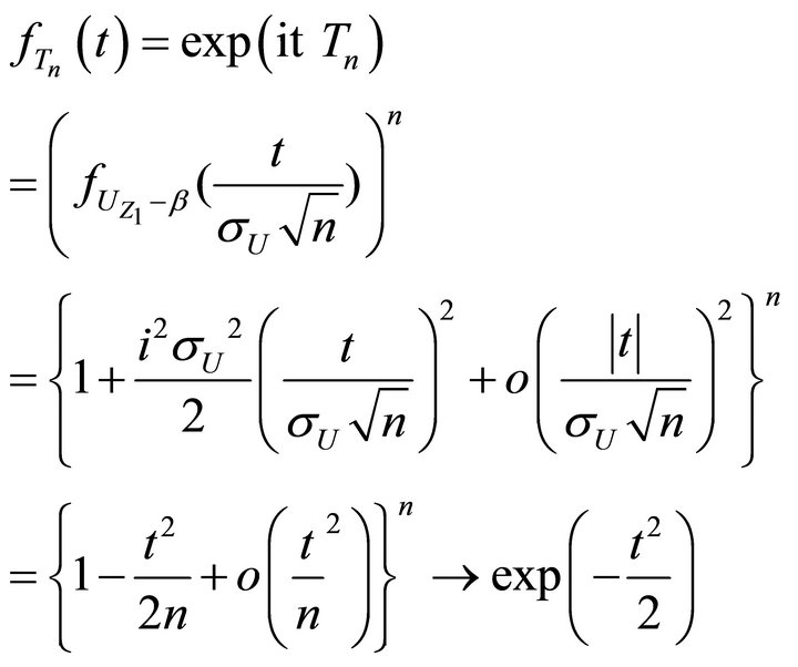
where the second equality comes from the Taylor expansion of . It is well known that this limit is the characteristic function of the random variable
  The same proof works for
 , using the components of the process
  as given in Theorem 3.12. ■
In some storage systems, the changes due to supply and release do not take place regularly in time. So it would be more realistic to consider the time parameter  as random. We will do so in what follows and will consider the asymptotic distributions of the processes
 , and
, and , when properly normalized and randomized. First let us put for each
 , and
, and
 .
.
Then we have:
4.4. Theorem: Let  be a sequence of integral valued random variables, independent of the
  and
and .
.
If  converges in probability to 1, as
 , then the randomized processes:
 and
and 
both converge in distribution to the Normal law 
Proof: It is a simple adaptation of [7], VIII.4, Theorem 4, p. 265. ■
5. Conclusion
In this paper, we presented a simple stochastic storage process  with a random walk input
  and a natural release rule
 . Realistic conditions are prescribed which make this process more tractable when compared to those models studied elsewhere (see Introduction). In particular the conditions led to a simple structure of random walk for the processes
  and
and , which has given explicitly their distributions, and a rather good insight on their asymptotic behavior since a SLLN and a CLT has been easily established for each of them. Moreover, a slightly more general limit theorem has been obtained when time is adequately randomized and both processes
  and
and  properly normalized.
6. Acknowledgements
I gratefully would like to thank the Referee for his appropriate comments which help to improve the paper.
REFERENCES
- E. Cinlar and M. Pinsky, “On Dams with Additive Inputs and a General Release Rule,” Journal of Applied Probability, Vol. 9, No. 2, 1972, pp. 422-429. doi:10.2307/3212811
- E. Cinlar and M. Pinsky, “A Stochastic Integral in Storage Theory,” Probability Theory and Related Fields, Vol. 17, No. 3, 1971, pp. 227-240. doi:10.1007/BF00536759
- J. M. Harrison and S. I. Resnick, “The Stationary Distribution and First Exit Probabilities of a Storage Process with General Release Rule,” Mathematics of Operations Research, Vol. 1, No. 4, 1976, pp. 347-358. doi:10.1287/moor.1.4.347
- J. M. Harrison and S. I. Resnick, “The Recurrence Classification of Risk and Storage Processes,” Mathematics of Operations Research, Vol. 3, No. 1, 1978, pp. 57-66. doi:10.1287/moor.3.1.57
- K. Yamada, “Diffusion Approximations for Storage Processes with General Release Rules,” Mathematics of Operations Research, Vol. 9, No. 3, 1984, pp. 459-470. doi:10.1287/moor.9.3.459
- P. A. Meyer, “Probability and Potential,” Hermann, Paris, 1975.
- W. Feller, “An Introduction to Probability Theory and Its Applications,” 2nd Edition, Wiley, Hoboken, 1970.