Applied Mathematics
Vol.3 No.10A(2012), Article ID:24091,8 pages DOI:10.4236/am.2012.330181
An Inexact Restoration Package for Bilevel Programming Problems
Facultad de Matemática, Astronomía y Física, Universidad Nacional de Córdoba, CIEM (CONICET), Córdoba, Argentina
Email: pilotta@famaf.unc.edu.ar, torres@famaf.unc.edu.ar
Received June 1, 2012; revised July 1, 2012; accepted July 8, 2012
Keywords: Bilevel Programming Problems; INEXACT Restoration Methods; Algorithms
ABSTRACT
Bilevel programming problems are a class of optimization problems with hierarchical structure where one of the constraints is also an optimization problem. Inexact restoration methods were introduced for solving nonlinear programming problems a few years ago. They generate a sequence of, generally, infeasible iterates with intermediate iterations that consist of inexactly restored points. In this paper we present a software environment for solving bilevel programming problems using an inexact restoration technique without replacing the lower level problem by its KKT optimality conditions. With this strategy we maintain the minimization structure of the lower level problem and avoid spurious solutions. The environment is a user-friendly set of Fortran 90 modules which is easily and highly configurable. It is prepared to use two well-tested minimization solvers and different formulations in one of the minimization subproblems. We validate our implementation using a set of test problems from the literature, comparing different formulations and the use of the minimization solvers.
1. Introduction
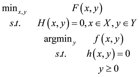
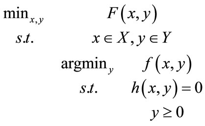
Bilevel programming problems are optimization problems whose feasible set is partially restricted to the solution of another optimization problem. Mathematically speaking, a bilevel problem can be stated by:
 (1)
(1)
where ,
,  ,
,  ,
, . Eventually, some components of vector y may be free. The sets X and Y are bounded boxes in
  and
and  respectively. We suppose that the gradients of F and H, and the Hessians of f and h exist and are continuous in X × Y. The optimization subproblem appearing in the constraints is called the lower level problem.
The first formulation of bilevel programming was given in an economical context in [1]. Survey papers on this problem were published in [2,3]. Different approaches about the theory of optimality conditions for bilevel programming problems were introduced in [4]. In [5,6] necessary and sufficient optimality conditions require that the lower level problem has a unique optimal solution.
Following Dempe [7] algorithms for solving bilevel programming problems can be classified into three categories: the first group solves the problem globally, the second group computes stationary points or points that satisfy some local optimality conditions, and the third group corresponds to heuristic methods. A review of algorithms for globally solving this kind of problems is given in [2].
Bilevel programming problems are nonconvex optimization problems and for this reason there are difficulties to solve them globally. Therefore, descent methods were developed to compute stationary solutions. For the linear case, see [8]. An important fact assumed in [9] is that the lower level optimal solution is uniquely determined.
The development of new algorithms and theory of bilevel programming problems is strongly motivated by a large number of applications. For instance, determination of optimal prices [10], aluminium production process [11], electric utility demand-side planning and engineering applications [12]. An overview of applications is given in [13].
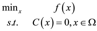
In order to solve bilevel programming problems we will consider the ideas proposed in [14-16], called Inexact Restoration methods (IR). Let us state the nonlinear programming problem in the form:
 (2)
(2)
where  and
and  are continuously differentiable and Ω is a polytope. The IR model algorithm generates feasible iterates with respect to Ω. Each iteration includes two different phases: restoration and minimization. In the restoration phase, which is executed once per iteration, an intermediate point (restored point) is found such that its infeasibility is a fraction of the infeasibility of the current point. After restoration we define a linearization of the feasible region πk around the restored point. In the minimization phase we compute a trial point belonging to πk solving a trust-region subproblem such that the functional value at the trial point is less than the functional value at the restored point. A Lagrangian function can be also used at the minimization phase as it is presented in [16,17]. By means of a merit function, the new iterate is accepted or rejected. In case of rejection, the trust-region radius is reduced and the minimization phase is repeated around the same restored point. The philosophy of IR encourages case-oriented applications. Since IR allows us to choose suitable restoration and minimization procedures, the IR approach is quite appealing in this context.
Many years ago bilevel programming problems were solved replacing the lower level problem by its KKT conditions, but this presented a serious drawback because many spurious stationary points may appear. On the other hand, one of the reasons for using IR in bilevel programming problems is that the lower level problem may be treated at the restoration phase as an optimization problem. The classical way to find a local solution is to try to solve the lower level problem using optimization strategies that consider the lower objective function. Besides that, notice that when Ω is a polytope, the approximate feasible region πk is also a polytope. Thus, the minimization phase consists of solving a linearly constrained optimization problem. Therefore, available algorithms for these kinds of (potentially large-scale) problems can be fully exploited, for example MINOS [18], SNOPT [19] and ALGENCAN [20].
Our main contribution is to propose a user-friendly environment consisting by a set of Fortran 90 modules to solve a bilevel programming problem using IR without reformulating it as a single-level problem. The package is easily and highly customizable and it is prepared to use two well-tested minimization solvers and different formulations in the minimization subproblem. Other solvers can be easily included with minor changes in the code. The algorithm is based on [6], with additional features: two versions for solving the minimization step and stopping criteria. One of the most attractive features of this environment is the autosetting options. That means that users just need to write Fortran code for the functions involved in the bilevel programming problem, and not to write any code about the algorithm and external solvers. On the other hand, the code is highly configurable, therefore users with expertise on these topics may take advantage of the code structure.
The code is written mainly in standard Fortran 90, with a few features of standard Fortran 2003. The choice of the language was made because a big number of optimization packages are written either in Fortran 77 or in Fortran 90. Particularly, MINOS and ALGENCAN are written in Fortran 77, which are used in our code.
We validate our implementation using a set of test problems from the literature, comparing different formulations and the use of the minimization solvers.
There are several formulations for the bilevel programming problem in the literature with their own code, but not software packages. For example, in [21] genetic algorithms are developed using GAMS [22] and MINOS, in [23] a decomposition based on global optimization approach to bilevel and quadratic programming problems is solved by GAMS/MINOS.
The most popular available package is BIPA (BIlevel Programming with Approximation methods) [24]. BIPA is a code written in C for solving nonlinear bilevel programming problems. It is a trust-region type method where the subproblem consists in solving a sequence of mixed-integer programs (MIPs) and nonlinear optimization problems. The latter programs are solved using ILOG CPLEX [25] routines and DONLP2 [26] respectively. ILOG CPLEX is a high-performance mathematical programming solver for linear programming, mixed-integer programming, and quadratic programming, and it is mantained by IBM. DONLP2 is a solver for general nonlinear programming problems.
The paper is structured as follows. In Section 2 a mathematical background of IR methods is given. Section 3 is devoted to explain an algorithm based on IR applied to solve bilevel programming problems. Section 4 refers to the design of the package, and Section 5 shows numerical experiments for a set of test problems. Finally, Section 6 is dedicated to the conclusions.
2. Inexact Restoration Methods
IR methods have been introduced in the last few years for solving nonlinear programming problems [14-16], due to the drawbacks present in feasible methods. Feasible methods generate a sequence of feasible points that, in the presence of strong nonlinearities, may behave badly. In these cases, it is not appropriate to perform large steps far from the solution, because the nonlinearity forces the distance between consecutive feasible iterates to be very short. On the other hand, short steps far from the solution are not convenient because it may produce slow convergence. IR methods keep infeasibility under control and are tolerant when the iterates are far from the solution. At the end of the algorithm feasibility is preserved since the weight of infeasibility is increased during the process.
IR methods are intended to solve the following problem
 (3)
(3)
where  and
and  are continuously differentiable and
  is a closed and convex set. Each iteration consists of two phases: restoration and minimization. In the restoration phase an intermediate point
  is obtained such that the infeasibility at yk is reduced with respect to the infeasibility at xk. At the beginning of the minimization phase a linearization πk of the feasible region defined by the constraints C(x) = 0 is constructed around the restored point yk, that is:
 (4)
(4)
Then, a trial point

is computed such that . Here
  is a trust-region radius. Another formulation [17] solves a minimization problem where the objective function is replaced by its Lagrangian function:
 (5)
(5)
for all . In order to accept the trial point
  a penalty merit function is considered:
 (6)
(6)
where  is a penalty parameter defined by a nonmonotone sequence. Instead of the merit function, a filter criterion may be considered to accept the trial point [27]. Until the acceptance condition is satisfied, the trust-region radius is reduced and the minimization problem is solved again.
The minimization phase is a problem with linear constraints (if Ω is a polytope), therefore any available solver for linearly constrained optimization can be applied. Besides that, the method gives the freedom to formulate each phase and choose the solver in order to take advantage of the structure of the problem. These features make the IR methods very attractive.
There exist convergence results for the sequence generated by the IR methods under mild hypotheses [14,15].
3. IR Bilevel Algorithm
Let us consider, without loss of generality, the following problem:
 (7)
(7)
We write the KKT conditions of the lower level problem in the form
 (8)
(8)
where  and
and . Based on [6] we propose the following algorithm:
3.1. Algorithm
Set the algorithmic parameters tol, M > 0,  ,
,  ,
,  , {wk} a summable sequence of positive numbers, and initial approximations x0, y0, γ0 and λ0 (initial Lagrangian multiplier estimators).
Step 1. At iteration k, set
 ,
,

Step 2. Restoration phase. Find yR, μRand γR such that
Step 3. Minimization phase. Set i ← 0 and choose  Compute a trial point
  as the solution of the following problem

For the Lagrangian formulation, change the objective function by the Lagrangian function
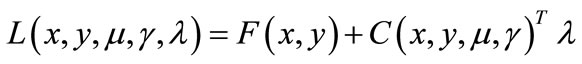
with .
.
Step 4. Update the Lagrangian multipliers (only for the Lagrangian formulation). Compute a trial  such that
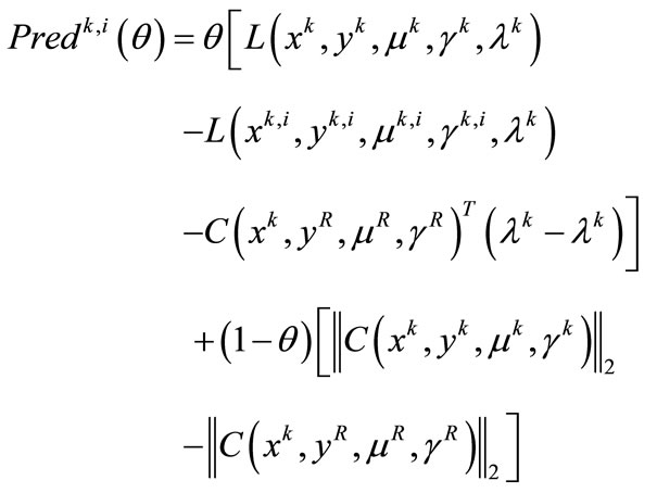
Step 5. Predicted reduction. Compute  as the maximum
  such that
where
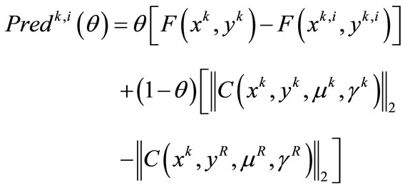
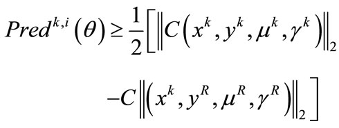
For the Lagrangian formulation the predicted reduction is defined by
Set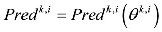 .
.
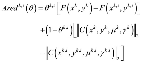
Step 6. Actual reduction. Compute
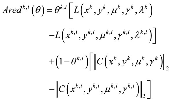
For the Lagrangian formulation, the actual reduction is defined by
Step 7. Acceptance and stopping criteria. See the algorithm described below.
3.2. Acceptance and Stopping Criteria
We wish that the merit function at the trial point should be less than the merit function at the current point, that is, . However, as in unconstrained optimization a reduction of the merit function is not enough to guarantee convergence. In fact, we need a sufficient reduction of the merit function, that is defined by the following test:

If this test holds, we accept the trial point as a new approximation and terminate iteration k. Otherwise, we reduce the trust-region radius and repeat the minimization phase.
The stopping criteria proposed here consists of a comparison between two successive approximations of either the sequence , or the sequence of functional values
 , and a feasibility test using the KKT conditions of the lower level problem and the upper level constraints (if there exist).
We remark that the new stopping criteria is different from the criteria used in [1], where a nonlinear minimization problem has to be solved in each iteration and this could be computationally expensive. Moreover, the numerical experiments validate the proposed procedure.
The proposed stopping criteria is:
if  then
then
set ,
,  and
and
repeat minimization phase (Step 3)
else
compute
set ,
,
 ,
, 
set 
if  or
or 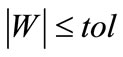 then
then
if 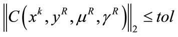 then
then
Terminate declaring finite convergence
Otherwise Return to restoration phase
(Step 2)
end
else
Return to restoration phase (Step 2)
end
end
4. Design
The software environment presented here consists of a set of modules, mainly in standard Fortran 90, that solves the bilevel programming problem using an IR formulation. The algorithm is based on the ideas of [6] with a new stopping criterion and two optional procedures for the minimization phase. The code is able to solve restoration and minimization phases by means of two optimization solvers: MINOS and ALGENCAN. MINOS has been extensively used for many years and it is one of the most known codes in optimization, becoming a reference in this area. Although MINOS is a commercial software, our code can be compiled using ALGENCAN instead of MINOS (ALGENCAN can be freely downloaded). Other solvers could be included with minor changes. Each problem can be configured in only one module with its own setting options (default or advanced) independently of the rest of the code. A list of capabilities is described below:
Modularity: the modules can be classified into categories: 1) sizes, bounds and initial conditions; 2) default algorithmic parameters like solver and formulation choices, tolerances, etc.; 3) variables of the external solvers; 4) variables from different phases; 5) definition of the problem (this is the only one module provided by the user); 6) modules related to the bilevel algorithm (completely independent of the problem and external solvers).
Simplicity: there are no derived types of variables defined in the code. The code has been prepared for both an expert programmer as well as for a medium programmer.
Language: the modules are programmed in standard Fortran 90 with a very few features of standard Fortran 2003 (for instance, array constructors) for easier data input. It has been successfully compiled and executed with the Intel Fortran Compiler, Portland Fortran Compiler, GNU Fortran and G95.
Configurability: there are two possible configurations: default and advanced. The default configuration only requires to set problem sizes, initial conditions and the functions involved in the problem. The advanced configuration needs the requirements of the default configuration and allows to modify one or several default parameters and procedures, for instance:
- external solver (MINOS or ALGENCAN);
- Lagrangian or non Lagrangian formulation;
- solver settings for restoration or minimization phases;
- function settings for restoration or minimization phases;
- KKT conditions of the lower level problem and the upper level constraints;
Precision: the code handles double precision real variables, because the external solvers (MINOS and ALGENCAN) handle double precision real variables by default.
5. Numerical Experiments
In this section we illustrate the use of our software to solve a particular bilevel programming problem. Besides that, we consider a set of test problems from the literature and present numerical results for different parameters and options of our code (i.e. external solvers, formulations, etc.).
5.1. Sample Application
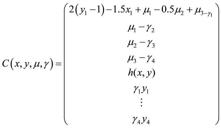
We consider the problem BIPA2 from [24]:
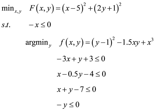
We add slack variables and rewrite the problem in the following standard form:
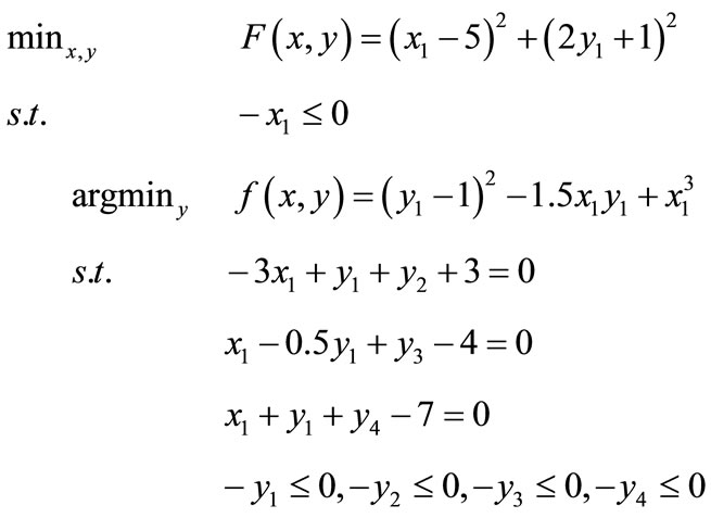
where x = (x1) and y = (y1, y2, y3, y4).
Specific settings may require additional information for the restoration and minimization phases, for example the calculation of the function  (see Equation (8)) representing the KKT conditions of the lower level problem and its Jacobian matrix
 :
:
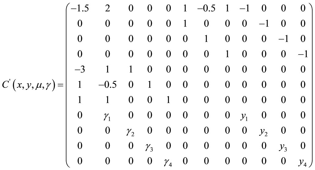
In order to avoid messy computations to obtain functions C and C', or the solver settings, users can choose the default configuration, in which only the problem data has to be given. In case of a complex problem, the default configuration is a good option to prevent human errors.
The next subsection contains a number of other examples. For programming details please refer to the user manual that accompanies the software.
5.2. Additional Test Problems
Table 1 reports test problems from literature. The first column indicates the problem as it is referenced in the last column. The numbers n, m, q and p are the same than in (1).
Most of these problems belong to the test problem collection in [28]. Initial points are given in Table 1. All tests were performed in a PC running Linux, Core 2 Duo, 2.0GHz, 3Gb RAM, with the following Fortran compilers: Intel Fortran Compiler, G95, GNU Fortran and Portland Compiler.
In all cases the solution was successfully found in a small number of iterations (except problem 9.2.05 that converged in 43 iterations) and agrees with the reported solution (see Table 2). Notice that these results were obtained using the default configuration. The main default setting parameters are:
- External solver: MINOS.
- IR formulation: without using the Lagrangian formulation.
- All of the solver dependent functions are automatically set.
For a complete list of setting parameters, please refer to the user manual.
All the problems in Table 2 were tested with advanced configurations, for example using a user setting function C. The same results were obtained using other formulations, for instance, ALGENCAN as the external solver and the Lagrangian function. The numerical results agree in all cases unless the number of iterations, due to internal formulations.
In all cases the CPU time was negligible, therefore no comparison with other solvers could be made.
6. Conclusions
The main idea behind this work is to provide an environment in order to solve general bilevel programming problems. One of the most important features of our implementation besides portability is to provide a userfriendly code. At the same time the code is intended to be highly configurable to exploit the best characteristics of both the problems and external solvers. This environment,
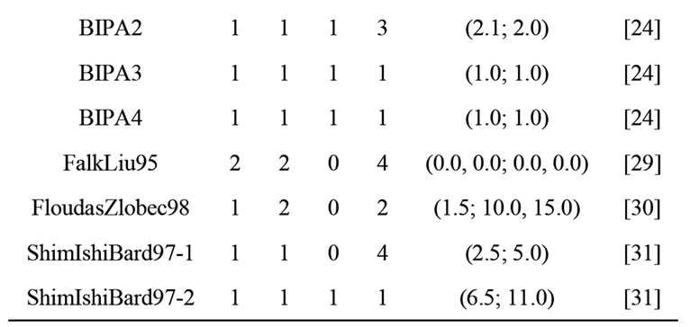
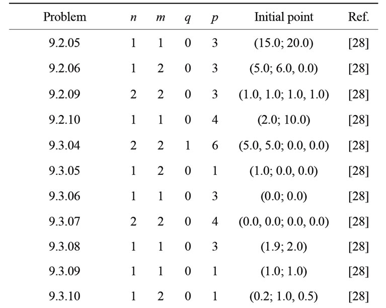
Table 1. Test problems.
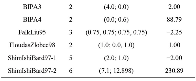
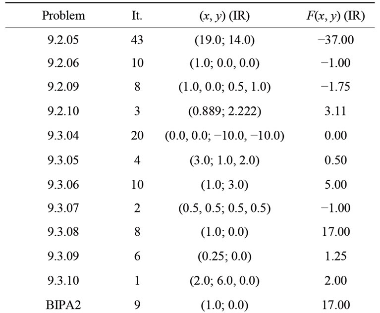
Table 2. Numerical experiments for test problems with the default configuration.
in the case of the default configuration, supplies all the necessary tools to automatically set the auxiliary subroutines and solvers. Therefore, it allows a cleaner and shorter coding and avoids a lot of human errors.
The bilevel algorithm based on the inexact restoration method has appealing theoretical properties, in the sense that under certain hypotheses, convergence is assured [1]. This feature is a remarkably advantage over other packages that solve bilevel programming problems without convergence results. To solve each phase of the inexact restoration algorithm adapted to bilevel programming problems, external solvers are needed. In our case we use two packages (MINOS and ALGENCAN), however, other solvers can be added with minor changes in the source code. We decided not to mix different solvers for the restoration and minimization phases, because they are based on different philosophies. For instance, MINOS uses factorizations and ALGENCAN exploits matrix-vector products.
Finally, numerical results are promising since different kinds of bilevel programming problems (linear, quadratic and nonlinear) have been successfully solved. Several tests have been carried out using different algorithmic parameters and configurations with the same results, with similar execution time.
The source code and the user manual can be obtained from the authors’ electronic addresses.
REFERENCES
- H. V. Stackelberg, “Marktform and Gleichgewicht,” Springer-Verlag, Berlin, 1934.
- J. F. Bard, “Practical Bilevel Optimization: Algorithms and Applications,” Kluwer Academic Publishers, Dordrecht, 1998.
- L. N. Vicente, “Bilevel Programming: Introduction, History, and Overview,” In: Encyclopedia of Optimization, Kluwer Academic Publishers, Dordrecht, 2001, pp. 24-31. doi:10.1007/0-306-48332-7_38
- S. Dempe, “Foundations of Bilevel Programming,” Kluwer Academic Publishers, Dordrecht, 2002.
- S. Dempe, “A Necessary and a Sufficient Optimality Condition for Bilevel Programming Problems,” Optimization, Vol. 25, No. 4, 1992, pp. 341-354. doi:10.1080/02331939208843831
- R. Andreani, S. L. C. Castro, J. L. Chela, A. Friedlander and S. A. Santos, “An Inexact-Restoration Method for Nonlinear Bilevel Programming Problems,” Computational Optimization and Applications, Vol. 43, No. 3, 2009, pp. 307-328. doi:10.1007/s10589-007-9147-4
- S. Dempe, “Annottated Bibliography on Bilevel Programming and Mathematical Problems with Equilibrium Constraints,” Optimization, No. 52. No. 3, 2003, pp. 333-359. doi:10.1080/0233193031000149894
- S. Dempe, “A Simple Algorithm for the Linear Bilevel Programming Problem,” Optimization, No. 18, No. 3, 1987, pp. 373-385. doi:10.1080/02331938708843247
- J. E. Falk and J. Liu, “Annotated Bibliography on Bilevel Programming and Mathematical Programs with Equilibrium Constraints,” Central European Journal of Operations Research, Vol. 52, No. 2, 1993, pp. 101-117.
- L. Brotcorne, M. Labbè, P. Marcotte and G. Savard, “A Bilevel Model and Solution Algorithm for a Freight Tariff Setting Problem,” Transportation Science, Vol. 34, No. 3, 2000, pp. 289-302. doi:10.1287/trsc.34.3.289.12299
- M. G. Nicholls, “The Application of Nonlinear Bilevel Programming to the Aluminium Industry,” Journal of Global Optimization, Vol. 8, No. 3, 1996, pp. 245-261. doi:10.1007/BF00121268
- J. Herskovits, A. Leontiev, G. Dias and G. Santos, “Contact Shape Optimization: A Bilevel Programming Approach,” Structural and Multidisciplinary Optimization, Vol. 20, No. 3, 2000, pp. 214-221.
- P. Marcotte and G. Savard, “Bilevel Programming: Applications,” In: Encyclopedia of Optimization, Kluwer Academic Publishers, Dordrecht, 2001. doi:10.1007/0-306-48332-7_33
- J. M. Martínez, “Two-Phase Model Algorithm with Global Convergence for Nonlinear Programming,” Journal of Optimization Theory and Applications, Vol. 96, No. 2, 1998, pp. 397-436. doi:10.1023/A:1022626332710
- J. M. Martínez and E. A. Pilotta, “Inexact Restoration Algorithm for Constrained Optimization,” Journal of Optimization Theory and Applications, Vol. 104, No. 1, 2000, pp. 135-163. doi:10.1023/A:1004632923654
- J. M. Martínez and E. A. Pilotta, “Inexact Restoration Methods for Nonlinear Programming: Advances and Perspectives,” In: L. Q. Qi, K. Teo and X. Q. Yang, Eds., Optimization and Control with Applications, Applied Optimization Series, Chapter 12, Springer, Netherlands, 2005, pp. 271-292.
- E. G. Birgin and J. M. Martínez, “Local Convergence of an Inexact-Restoration Method and Numerical Experiments,” Journal of Optimization Theory and Applications, Vol. 127, No. 2, 2005, pp. 229-247. doi:10.1007/s10957-005-6537-6
- B. A. Murtagh and M. A. Saunders, “Large-Scale Linearly Constrained Optimization,” Mathematical Programming, Vol. 14, No. 1, 1978, pp. 41-72. doi:10.1007/BF01588950
- W. Murray, P. E. Gill and M. A. Saunders, “SNOPT: An SQP Algorithm for Large-Scale Constrained Optimization,” SIAM Journal on Optimization, Vol. 12, No. 4, 2002, pp. 979-1006.
- E. G. Birgin and J. M. Martínez, “Large-Scale Active-Set Box-Constrained Optimization Method with Spectral Projected Gradients,” Computational Optimization and Applications, Vol. 23, No. 1, 2002, pp. 101-125. doi:10.1023/A:1019928808826
- S. R. Hejazi, A. Memariani, G. Jahanshahloo and M. M. Sepehri, “Linear Bilevel Programming Solution by Genetic Algorithm,” Computers & Operations Research, Vol. 29, No. 13, 2002, pp. 1913-1925. doi:10.1016/S0305-0548(01)00066-1
- GAMS, http://www.gams.com/
- V. Visweswaran, C. A. Floudas, M. G. Ierapetritou and E. N. Pistikopoulos, “State of the Art in Global Optimization: Computational Methods and Applications,” Kluwer Academic Publishers, Dordrecht, 1996.
- B. Colson, P. Marcotte and G. Savard, “A Trust-Region Method for Nonlinear Bilevel Programming: Algorithm and Computational Experience,” Computational Optimization and Applications, Vol. 30, No. 3, 2005, pp. 211- 227. doi:10.1007/s10589-005-4612-4
- CPLEX. http://www-01.ibm.com/software/integration/optimization/cplex-optimizer/
- P. Spellucci, “An SQP Method for General Nonlinear Programs Using Only Equality Constrained Subproblems,” Mathematical Programming, Vol. 82, No. 3, 1998, pp. 413-448. doi:10.1007/BF01580078
- E. Karas, E. Pilotta and A. Ribeiro, “Numerical Comparison of Merit Function with Filter Criterion in Inexact Restoration Algorithms Using Hard-Spheres Problems,” Computational Optimization and Applications, Vol. 44, No. 3, 2009, pp. 427-441. doi:10.1007/s10589-007-9162-5
- C. A. Floudas, P. M. Pardalos, C. S. Adjiman, W. R. Esposito, Z. Gumus, S. T. Harding, J. L. Klepeis, C. A. Meyer and C. A. Schweiger, “Handbook of Test Problems for Local and Global Optimization,” Kluwer Academic Publishers, Dordrecht, 1999. doi:10.1007/BF01585928
- J. E. Falk and J. Liu, “On Bilevel Programming, Part I: General Nonlinear Cases,” Mathematical Programming, Vol. 70, No. 1, 1995, pp. 47-72.
- Z. H. Gumus and C. A. Floudas, “Global Optimization of Nonlinear Bilevel Programming Problems,” Journal of Global Optimization, Vol. 20, No. 1, 2001, pp. 1-31. doi:10.1023/A:1011268113791
- K. Shimizu, Y. Ishizuka and J. F. Bard, “Nondifferentiable and Two-Level Mathematical Programming,” Kluwer Academic Publishers, 1997. doi:10.1007/978-1-4615-6305-1