Applied Mathematics
Vol. 3 No. 6 (2012) , Article ID: 20080 , 7 pages DOI:10.4236/am.2012.36080
A Nonstandard Finite Difference Scheme for SIS Epidemic Model with Delay: Stability and Bifurcation Analysis
Department of Mathematics, Faculty of Sciences, Brawijaya University, Malang, Indonesia
Email: suryanto@ub.ac.id
Received March 22, 2012; revised April 22, 2012; accepted May 5, 2012
Keywords: SIS Epidemic Model with Delay; Stability; Nonstandard Finite Difference Method; Neimark-Sacker (Hopf) Bifurcation
ABSTRACT
A numerical scheme for a SIS epidemic model with a delay is constructed by applying a nonstandard finite difference (NSFD) method. The dynamics of the obtained discrete system is investigated. First we show that the discrete system has equilibria which are exactly the same as those of continuous model. By studying the distribution of the roots of the characteristics equations related to the linearized system, we can provide the stable regions in the appropriate parameter plane. It is shown that the conditions for those equilibria to be asymptotically stable are consistent with the continuous model for any size of numerical time-step. Furthermore, we also establish the existence of Neimark-Sacker bifurcation (also called Hopf bifurcation for map) which is controlled by the time delay. The analytical results are confirmed by some numerical simulations.
1. Introduction
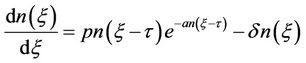
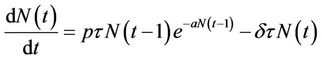
In this paper we reconsider a SIS epidemic model with maturation delay developed in [1]:
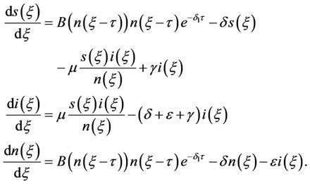 (1)
(1)
Here  is a birth rate function. The size of mature population
  at time
  is divided into susceptible
  and infective
  classes, so that
  .
. ,
,  are the death rates of immature and mature population, respectively. The delay
  is considered as the maturation time. The parameter
 ,
,  and
and  are respectively the constant contact rate, the disease induced death rate constant and the recovery constant rate, respectively.
In this paper we consider a special class of Equation (1) by assuming that the death rate in each stage prior to the adult stage and the disease induced death are negligible, i.e. . Using the Rick function as the birth rate function
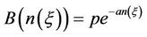 , Equation (1) becomes
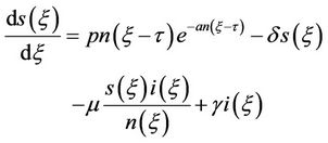 (2.a)
(2.a)
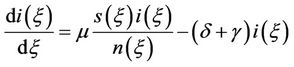 (2.b)
(2.b)
 (2.c)
(2.c)
Note that Equation (2.c) is decoupled and is called the Nicholson’s blowflies equation which proposed by [2]. The dynamics of Equation (2.c) have been studied by many authors; see e.g. [3,4].
In [1], the basic reproduction number for system (2) has been identified as
 . (3)
. (3)
It has also been shown in [1] that  determines the existence of equilibria as well as their stability properties. They have shown numerically that if the delay
  is sufficiently large then the positive solutions of system (2) oscillate about the positive equilibrium. The existence and stability of Hopf bifurcation were established by Wei and Zou [5]. In this case, the bifurcation is controlled by parameter p. The bifurcation analysis of system (2) using time delay as the control parameter has been done by Chi, Qu and Wei [6].
For practical purposes, we need to do numerical simulations and therefore we have to transform the continuous model (2) into a discrete system. We expect that the dynamical properties of the discrete system are in accordance with its continuous counterpart (2). Kunnawuttipreechachan [7] and the author [8] considered the Euler discretization of system (2) and showed that the discrete system has exactly the same equilibria as those of system (2). Using different method of analysis, Kunnawuttipreechachan [7] and the author [8] derived the sufficient conditions of the numerical step-size for equilibria to be asymptotically stable. It was concluded that the stability conditions of equilibria of the discrete system obtained by the Euler method are consistent with system (2) only if the numerical time-step is relatively small.
To overcome the dependence of stability condition on the time-step size, we will apply a nonstandard finite difference (NSFD) scheme. This method, which is developed by Mickens [9,10], has been applied to various problems; see e.g. [11-16], in which the numerical solutions preserve dynamical properties of the continuous model. We will show that the discrete SIS epidemic model with a delay obtained by the NSFD method maintains the stability properties of equilibria irrespective of the size of numerical time-step. Besides the stability conditions, the existence of bifurcation of the discrete model will also be investigated.
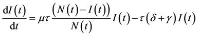
2. Discrete SIS Epidemic Model with Delay
Using the fact that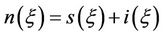 , we will only consider the last two equations of system (2). Using a transformation
  and
and 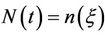 with
with , Equation (2.b) and (2.c) can be written as
 (4.a)
(4.a)
 (4.b)
(4.b)
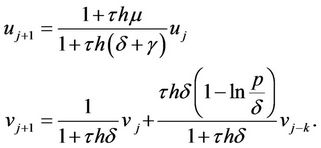
To discretize system (4) we first consider the step-size of the form  where k is a positive integer. Then, applying the forward difference scheme for the derivative and a nonlocal approximation for the right hand sides of system (4) yields a system of difference equations
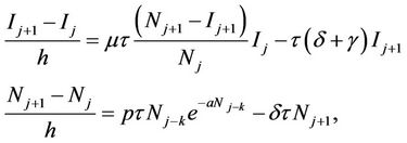 (5)
(5)
where  and
and  are numerical approximation of
  and
and 
 , respectively. The numerical scheme (5) is a nonstandard because it uses a nonlocal approximation; see Mickens [9,10]. Here we consider initial conditions
 and
and ,(6)
,(6)
where , for
, for . It is easy to show that the implicit scheme (5) can be arranged to get its explicit version, i.e.
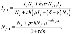 (7)
(7)
Direct calculations show that the discrete system (7) has a unique equilibrium: 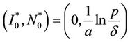 if
if 
and . This equilibrium is called the disease free equilibrium (DFE). On the other hand, if
  and
and  then, in addition to the DFE, there also exists an endemic equilibrium (EE):
  where
where
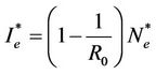 and
and .
.
We observe that those equilibria are exactly the same as those of the continuous system (4); see e.g. [7].
3. Stability and Neimark-Sacker Bifurcation Analysis
It is well known that the stability of equilibrium of a dynamical system depends on the distribution of the zeros of its associated characteristics equation. In this section, the distribution of the roots of the characteristics equation will be analyzed using the following results of Zhang, Zu and Zheng [17].
Theorem 1 (Zhang, Zu and Zheng [17]).
Suppose that  is a bounded, closed and connected set;
 is continuous in
  and
and  is a parameter. Then as
  varies, the sum of the order of the zeros of
  out of the unit circle:
can change only if a zero appears on or crosses the unit circle.
3.1. Disease Free Equilibrium
First we perform a linearization of system (7) about the DFE  by taking
  and
and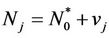 . The linearized system around the DFE is given by
 (8)
(8)
By introducing new variables
 we can rewrite system (8) in the form
 (9)
(9)
where 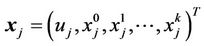 and the constant matrix A is defined by
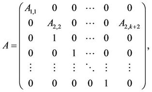
with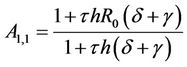 ,
, 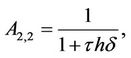 and
and 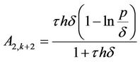 . The characteristic equation of matrix A is
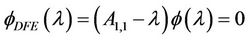 (10)
(10)
where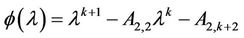 .
.
Lemma 1. If  and
and  then there exists a
  such that all roots of Equation (10) have modulus less than one for
 .
.
Proof. The trivial root of Equation (10) is
 .
.
It is clear that if  then
then  for all
 . Other roots of Equation (10) are determined by
 . (11)
when , Equation (11) becomes
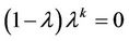 .
.
Hence Equation (11), at , has a root
  of multiplicity k and a simple root
 . Consider the root
  such that
 . This root depends continuously on
 . Based on Equation (11) we have
 (12)
(12)
whenever . Consequently all roots of Equation (10) lie in
  for all sufficiently small
 , and the existence of the maximal
  follows.
Lemma 2. If  then Equation (11) has no root with modulus one for all
 .
.
Proof. Assume  with
with  be a root of Equation (11) when
 . Substituting this root to Equation (11) yields
 .
.
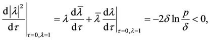
Separating the real and imaginary parts, we have
 (13)
(13)
and therefore we get
 . (14)
If  then
then , which yields a contradiction. This completes the proof.
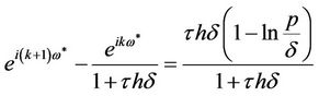
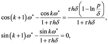
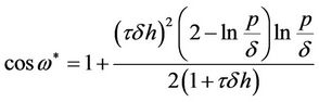
If , then the roots
  of Equation (11) with modulus one satisfy
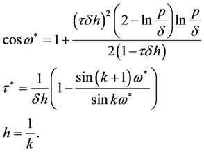 (15)
(15)
Lemma 3. If  then the roots of Equation (11) satisfy

where  and
and  satisfy Equation (15).
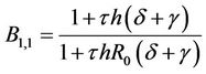
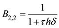
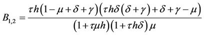
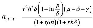
Proof. From Equations (11) and (15) we have

where
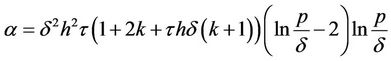
and
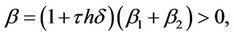
with
It is clear that if  then
then  and therefore
 .
.
Based on Theorem 1 and Lemmas 1-3, we have the following results on stability and bifurcation of system (5) at the DFE.
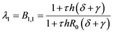
Theorem 2.
1) If  and
and  then the DFE is asymptotically stable for all
 .
.
2) If  and
and  then there exists an infinite sequence of time delay parameter
  such that the DFE is asymptotically stable when
  and unstable when
 . Map (7) has a Neimark-Sacker bifurcation at the DFE when
 ,
,  where
where  satisfy Equation (15).
Proof.
1) Let  and
and  then it is known from Lemmas 1 and 2 that the characteristic Equation (10) has no root with modulus one for all
 . Applying Theorem 1, all roots of Equation (10) have modulus less than one for all
 . Thus, conclusion (a) follows.
2) Let  and
and . It is known from Lemma 1 that if
  then one of roots of characteristics Equation (10) has modulus less than one for all
 . Other roots of Equation (10) satisfy Equation (11). From Lemmas 1 and 3 we know that all roots of Equation (11) have modulus less than one when
 , and Equation (11) has at least a couple of roots with modulus greater than one when
 . Hence conclusion (b) follows.
3.2. Endemic Equilibrium
The linearization of system (7) around the EE  is performed by substituting
  and
and  into system (7) to get
 (16)
(16)
where
 ,
,
 ,
,
 ,
,
and
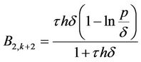 .
.
Using the same transformation as in the DFE, i.e.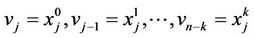 , system (16) can be written as
 (17)
(17)
where . The constant matrix B in Equation (17) is
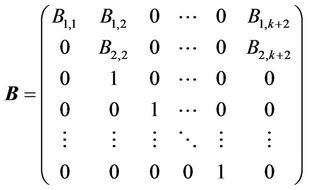 .
.
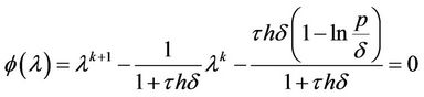
It is easy to show that the characteristic equation of matrix B is
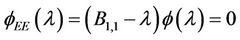 (18)
(18)
where 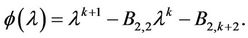 Clearly this characteristic equation has a trivial root
and other roots are determined by . Direct calculations show that if
  then
then  for all
 . Since
  and
and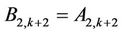 ,
,  is exactly the same as in Equation (11) and therefore the distribution of its roots is exactly the same as described by Lemmas 1-3. Hence we directly have the following results.
Lemma 4. If  and
and  then there exists a
  such that all roots of Equation (18) have modulus less than one for
 .
.
Lemma 5. If  and
and  then Equation (18) has no root with modulus one for all
 .
.
Lemma 6. If  and
and  then the modulus of trivial root of Equation (18), i.e.
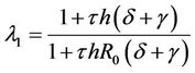 , is less than one for all
  and other roots satisfy
where  and
and  satisfy Equation (15).
Theorem 3.
1) If  and
and  then the EE is asymptotically stable for all
 .
.
2) If  and
and  then there exists an infinite sequence of time delay parameter
  such that the EE is asymptotically stable when
  and unstable when
 . System (7) has a Neimark-Sacker bifurcation at the EE when
 ,
,  where
where  satisfy Equation (15).
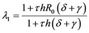
Theorems 2.1 and 3.1 give the sufficient conditions for DFE and EE to be asymptotically stable, respectively. Unlike the discrete system obtained by the Euler method where the stability conditions for equilibria depend on the size of time-step h, the proposed discrete system (7) has stability conditions which are consistent with the stability conditions for equilibria of continuous system (4) for any size of time step h; see [7] for the stability properties of the continuous system. In addition, Theorems 2.2 and 3.2 show the existence of bifurcation controlled by the time delay .
.
4. Numerical Simulations
To confirm our previous theoretical analysis, in this section we present some numerical simulations using nonstandard finite difference scheme (7) with time – step h = 0.1 (or k = 10). For the simulations we adopt parameters used by [7], i.e. ,
,  and
and . For the simulations of DFE and EE scenarios we use
  and
and , respectively.
4.1. Disease Free Equilibrium (R0 < 1)
For simulations of the DFE scenario we use a constant contact rate  and vary the value of p. Using this constant contact rate we have that
 . First we choose
  and therefore the conditions for the DFE to be stable are satisfied, i.e.
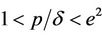 . Figure 1 shows the numerical solutions using
  and
and . It is indicated that the numerical solutions are convergent to the DFE (0.0, 0.9523) for any
 . On the other hand, if we take
  (i.e.,
 ) and other parameters are the same as used in Figure 1 then according to the previous analysis the DFE is unstable and the system undergoes a periodic solution of bifurcation. In this case the bifurcation point is
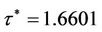 . Such behavior is shown in Figure 2. Indeed, if
 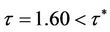 then the numerical solution converges to the DFE (0.0, 1.3064). On the contrary, the numerical solution, especially N(t), changes its stability from asymptotic stable to periodic behavior when
 .
.
4.2. Endemic Equilibrium (R0 > 1)
For the EE scenario we use  such that R0 = 2.3810 > 1. Figures 3(a) and (b) show the numerical solutions for
 (i.e
(i.e ), using
  and
and , respectively. These results indicate that if
  then the EE (0.5524, 0.9523) is asymptotically stable irrespective of
 .
.
Next we take the same parameters as used in Figure 3 but with , i.e.
 . Theorem 3 predicts that a Neimark-Sacker bifurcation will occur. From Equation (15) we find that the critical delay (bifurcation point) is
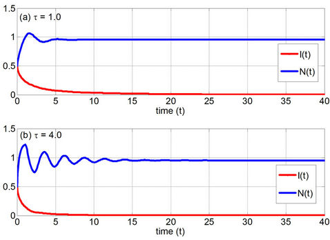
Figure 1. The numerical solutions of the discrete SIS model with a delay for the DFE scenario (R0 < 1) where 1 < p/δ < e2 and (a) τ = 1.0 and (b) τ = 4.0.
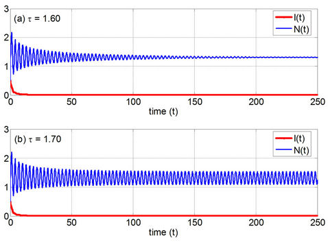
Figure 2. The numerical solutions of the discrete SIS model with a delay for the DFE scenario with p/δ > e2, R0 < 1 using (a) τ = 1.60 and (b) τ = 1.70.
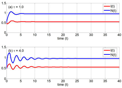
Figure 3. The numerical solutions of the discrete SIS model with a delay for the EE scenario with 1 < p/δ < e2 and R0 > 1 using (a) τ = 1.0 and (b) τ = 4.0.
 . This prediction is confirmed by our numerical solutions; see Figure 4. It is clearly seen that if we change the time delay from
  to τ = 1.70 >
 , then the behavior of numerical solutions changes from a solution converging to the EE (0.7577, 1.3064) to a solution which oscillates periodically about the EE.
Finally we compare the numerical solutions obtained by Euler method with those obtained by our NSFD method. We found that Euler method with a relatively big numerical time-step (h) may produce unrealistic negative and unbounded solutions. However, using the same or even bigger numerical time-step, NSFD method always gives positive and bounded solution. Depending on the parameters used in the simulations, the solution will be periodic or convergent to a correct equilibrium point. For example, in Figure 5 we plot the results of Euler method and NSFD method for the EE scenario using h = 0.25. It is seen from Figure 5(a) that the
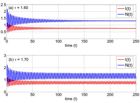
Figure 4. The numerical solutions of the discrete SIS model with a delay for the EE scenario with p/δ > e2, R0 > 1 using (a) τ = 1.60 and (b) τ = 1.70.
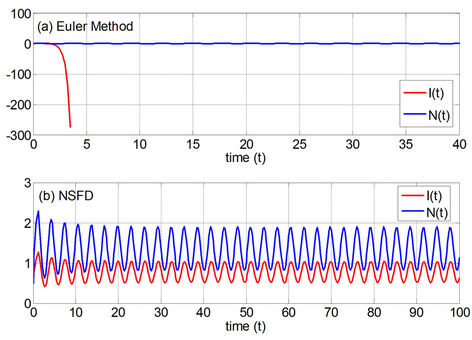
Figure 5. The numerical solutions for the EE scenario with p/δ > e2, R0 > 1, h = 0.25 (k = 4) and τ = 2 obtained by (a) Euler method and (b) NSFD method. Note that the result of Euler method is plotted in logarithmic scaled.
number of infectives tends to negative infinity (notice that the graph is shown in logarithmic scaled). Using the same value of h the solution of NSFD method oscillates about the EE; see Figure 5(b).
5. Conclusion
In this paper we have introduced a discrete delayed SIS epidemic model obtained by a nonstandard finite difference method. Unlike the Euler method, the proposed scheme reproduces exactly the same equilibria as well as their stability conditions as those of continuous model, i.e. if 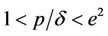 then the delay does not affect the stability of the equilibria. However, in the case of
 , the stability of equilibria changes when the delay passes a critical value. Here the discrete SIS model with a delay has periodic solutions when the stability is lost. In other words, a Neimark-Sacker bifurcation occurs. It is also shown that our numerical simulations have confirmed our analytical findings.
6. Acknowledgements
This research is supported by Direktorat Penelitian dan Pengabdian kepada Masyarakat, Direktorat Jenderal Pendidikan Tinggi Indonesia (Penelitian Unggulan Perguruan Tinggi—Fundamental) via DIPA Brawijaya University No. 0636/023-04.2.16/15/2012. The author would like to thank the anonymous reviewers for their valuable comments and suggestions to improve this article.
REFERENCES
- K. L. Cooke, P. V. D. Driessche and X. Zou, “Interaction of Maturation Delay and Nonlinear Birth in Population and Epidemic Model,” Journal of Mathematical Biology, Vol. 39, No. 4, 1999, pp. 332-352. doi:10.1007/s002850050194
- W. S. C. Gurney, S. P. Blythe and R. M. Nisbet, “Nicholson’s Blowflies (Revisited),” Nature, Vol. 287, No. 5777, 1980, pp. 17-21. doi:10.1038/287017a0
- J. Wei and M. Y. Li, “Hopf Bifurcation Analysis in a Delayed Nicholson Blowflies Equation,” Nonlinear Analysis, Vol. 60, No. 7, 2005, pp. 1351-1367. doi:10.1016/j.na.2003.04.002
- X. Ding and W. Li, “Stability and Bifurcation of Numerical Discretization Nicholson Blowflies Equation with Delay,” Discrete Dynamics in Nature and Society, Vol. 2006, 2006, pp. 1-12. http://www.hindawi.com/journals/ddns/2007/092959/ref/
- J. Wei and X. Zou, “Bifurcation Analysis of a Population Model and the Resulting SIS Epidemic Model with Delay,” Journal of Computational and Applied Mathematics, Vol. 197, No. 1, 2006, pp. 169-187. doi:10.1016/j.cam.2005.10.037
- Q. Chi, Y. Qu and J. Wei, “Bifurcation Analysis of an Epidemic Model with Delay as the Control Variable,” Applied Mathematics E-Notes, Vol. 9, 2009, pp. 307-319. http://www.math.nthu.edu.tw/~amen/2009/091020-2.pdf
- E. Kunnawuttipreechachan, “Stability of a Numerical Discretization Scheme for the SIS Epidemic Model with a Delay,” Proceedings of the World Congress on Engineering, London, Vol. 3, 30 June-2 July 2010, pp. 1923- 1930. http://www.iaeng.org/publication/WCE2010/WCE2010_pp1923-1930.pdf
- A. Suryanto, “Stability and Bifurcation of a Discrete SIS Epidemic Model with a Delay,” Proceedings of the 2nd International Conference on Basic Sciences, Malang, 24-25 February 2012, pp. 1-6.
- R. E. Mickens, “Application of Nonstandard Finite Difference Schemes,” World Scientific Publishing Co Pte. Ltd., Singapore City, 2000. doi:10.1142/9789812813251
- R. E. Mickens, “Numerical Integration of Population Models Satisfying Conservation Laws: NSFD Methods,” Journal of Biological Dynamics, Vol. 1, No. 4, 2007, pp. 427-436. doi:10.1080/17513750701605598
- D. T. Dimitrov and H. V. Kojouharov, “Nonstandard Finite Difference Method for Predator-Prey Models with General Functional Response,” Mathematics and Computers in Simulation, Vol. 78, No. 1, 2008, pp. 1-11. doi:10.1016/j.matcom.2007.05.001
- A. J. Arenas, J. A. Morano and J. C. Cortés, “Non-Standard Numerical Method for a Mathematical Model of RSV Epidemiological Transmission,” Computers and Mathematics with Applications, Vol. 56, No. 3, 2008, pp. 670-678. doi:10.1016/j.camwa.2008.01.010
- L. Jódar, R. J. Villanueva, A. J. Arenas and G. C. González, “Nonstandard Numerical Methods for a Mathematical Model for Influenza Disease,” Mathematics and Computers in Simulation, Vol. 79, No. 3, 2008, pp. 622- 633. doi:10.1016/j.matcom.2008.04.008
- A. J. Arenas, G. González-Parra and B. M. Chen-Charpentier, “A Nonstandard Numerical Scheme of Predictor-Corrector Type for Epidemic Models,” Computers and Mathematics with Applications, Vol. 59, No. 12, 2010, pp. 3740-3749. doi:10.1016/j.camwa.2010.04.006
- A. Suryanto, “A Dynamically Consistent Nonstandard Numerical Scheme for Epidemic Model with Saturated Incidence Rate,” International Journal of Mathematics and Computation, Vol. 13, No. D11, 2011, pp. 112-123. http://ceser.in/ceserp/index.php/ijmc/article/view/1151
- A. Suryanto, “A Dynamically Consistent Numerical Method for SIRS Epidemic Model with Non-Monotone Incidence Rate,” Proceedings of the 7th International Conference on Mathematics, Statistics and Its Application, Bangkok, 7-10 December 2011, pp. 273-282.
- C. Zhang, Y. Zu and B. Zheng, “Stability and Bifurcation of a Discrete Red Blood Cell Survival Model,” Chaos, Solitons and Fractal, Vol. 28, No. 2, 2006, pp. 386-394. doi:10.1016/j.chaos.2005.05.042.